Client Dask pour les ensembles de données plus volumineux

Dans cette section, nous allons analyser un ensemble de données plus vaste sur plusieurs intervalles de temps. Nous utiliserons le tableau de bord du client Dask pour visualiser l’état de nos calculs.

Cette section s’appuie sur les compétences des deux sections précédentes, notamment le chargement différé des données, l’ajout de plusieurs tâches à l’aide de « .compute() » et la visualisation du graphique des tâches à l’aide de « .visualise() ».

Charger des paquets

import datacube
import matplotlib.pyplot as plt
from deafrica_tools.dask import create_local_dask_cluster
from deafrica_tools.plotting import rgb, display_map

Connexion au datacube

dc = datacube.Datacube(app='Step3')

Créer un cluster Dask

create_local_dask_cluster()

/usr/local/lib/python3.8/dist-packages/distributed/node.py:151: UserWarning: Port 8787 is already in use.
Perhaps you already have a cluster running?
Hosting the HTTP server on port 42079 instead
  warnings.warn(

Client Scheduler: tcp://127.0.0.1:46737 Dashboard: /user/mseehaber@frontiersi.com.au/proxy/42079/status

Cluster Workers: 1 Cores: 4 Memory: 28.14 GB

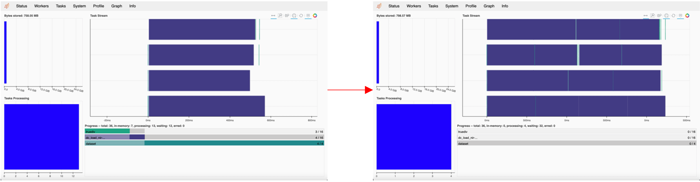
En retournant ceci, vous obtiendrez des informations sur le client et le cluster. Pour cet exercice, nous utiliserons le lien hypertexte vers le tableau de bord. Ce lien vous permettra de visualiser la progression de vos calculs au fur et à mesure de leur exécution.

Pour afficher le tableau de bord Dask et votre bloc-notes actif en même temps, suivez l’hyperlien et ouvrez-le dans une nouvelle fenêtre.

Chargement différé des données

lazy_data = dc.load(product='gm_s2_semiannual',
                   measurements=['blue','green','red','nir'],
                   x=(30.1505, 30.4504),
                   y=(30.0899, 30.3898),
                   time=('2020-01-01', '2021-12-31'),
                   dask_chunks={'time':1,'x':1500, 'y':1700})

lazy_data

<xarray.Dataset>
Dimensions:      (time: 4, y: 3317, x: 2895)
Coordinates:
  * time         (time) datetime64[ns] 2020-03-31T23:59:59.999999 ... 2021-09...
  * y            (y) float64 3.702e+06 3.702e+06 ... 3.669e+06 3.669e+06
  * x            (x) float64 2.909e+06 2.909e+06 ... 2.938e+06 2.938e+06
    spatial_ref  int32 6933
Data variables:
    blue         (time, y, x) uint16 dask.array<chunksize=(1, 1700, 1500), meta=np.ndarray>
    green        (time, y, x) uint16 dask.array<chunksize=(1, 1700, 1500), meta=np.ndarray>
    red          (time, y, x) uint16 dask.array<chunksize=(1, 1700, 1500), meta=np.ndarray>
    nir          (time, y, x) uint16 dask.array<chunksize=(1, 1700, 1500), meta=np.ndarray>
Attributes:
    crs:           EPSG:6933
    grid_mapping:  spatial_ref

xarray.Dataset

• Dimensions:
  • time: 4
  • y: 3317
  • x: 2895
• Coordinates: (4)
  • time
    (time)
    datetime64[ns]
    2020-03-31T23:59:59.999999 ... 2...

    units :

    seconds since 1970-01-01 00:00:00

    array(['2020-03-31T23:59:59.999999000', '2020-09-30T23:59:59.999999000',
           '2021-04-01T11:59:59.999999000', '2021-09-30T23:59:59.999999000'],
          dtype='datetime64[ns]')

  • y
    (y)
    float64
    3.702e+06 3.702e+06 ... 3.669e+06

    units :

    metre

    resolution :

    -10.0

    crs :

    EPSG:6933

    array([3701915., 3701905., 3701895., ..., 3668775., 3668765., 3668755.])

  • x
    (x)
    float64
    2.909e+06 2.909e+06 ... 2.938e+06

    units :

    metre

    resolution :

    10.0

    crs :

    EPSG:6933

    array([2909105., 2909115., 2909125., ..., 2938025., 2938035., 2938045.])

  • spatial_ref
    ()
    int32
    6933

    spatial_ref :

    PROJCS["WGS 84 / NSIDC EASE-Grid 2.0 Global",GEOGCS["WGS 84",DATUM["WGS_1984",SPHEROID["WGS 84",6378137,298.257223563,AUTHORITY["EPSG","7030"]],AUTHORITY["EPSG","6326"]],PRIMEM["Greenwich",0,AUTHORITY["EPSG","8901"]],UNIT["degree",0.0174532925199433,AUTHORITY["EPSG","9122"]],AUTHORITY["EPSG","4326"]],PROJECTION["Cylindrical_Equal_Area"],PARAMETER["standard_parallel_1",30],PARAMETER["central_meridian",0],PARAMETER["false_easting",0],PARAMETER["false_northing",0],UNIT["metre",1,AUTHORITY["EPSG","9001"]],AXIS["Easting",EAST],AXIS["Northing",NORTH],AUTHORITY["EPSG","6933"]]

    grid_mapping_name :

    lambert_cylindrical_equal_area

    array(6933, dtype=int32)

• Data variables: (4)
  • blue
    (time, y, x)
    uint16
    dask.array<chunksize=(1, 1700, 1500), meta=np.ndarray>

    units :

    1

    nodata :

    0

    crs :

    EPSG:6933

    grid_mapping :

    spatial_ref

    Array Chunk Bytes 76.82 MB 5.10 MB Shape (4, 3317, 2895) (1, 1700, 1500) Count 20 Tasks 16 Chunks Type uint16 numpy.ndarray

  • green
    (time, y, x)
    uint16
    dask.array<chunksize=(1, 1700, 1500), meta=np.ndarray>

    units :

    1

    nodata :

    0

    crs :

    EPSG:6933

    grid_mapping :

    spatial_ref

    Array Chunk Bytes 76.82 MB 5.10 MB Shape (4, 3317, 2895) (1, 1700, 1500) Count 20 Tasks 16 Chunks Type uint16 numpy.ndarray

  • red
    (time, y, x)
    uint16
    dask.array<chunksize=(1, 1700, 1500), meta=np.ndarray>

    units :

    1

    nodata :

    0

    crs :

    EPSG:6933

    grid_mapping :

    spatial_ref

    Array Chunk Bytes 76.82 MB 5.10 MB Shape (4, 3317, 2895) (1, 1700, 1500) Count 20 Tasks 16 Chunks Type uint16 numpy.ndarray

  • nir
    (time, y, x)
    uint16
    dask.array<chunksize=(1, 1700, 1500), meta=np.ndarray>

    units :

    1

    nodata :

    0

    crs :

    EPSG:6933

    grid_mapping :

    spatial_ref

    Array Chunk Bytes 76.82 MB 5.10 MB Shape (4, 3317, 2895) (1, 1700, 1500) Count 20 Tasks 16 Chunks Type uint16 numpy.ndarray

• Attributes: (2)

  crs :

  EPSG:6933

  grid_mapping :

  spatial_ref

Plusieurs tâches à l’aide de .compute()

Dans cette section, vous allez enchaîner plusieurs étapes pour calculer une nouvelle bande pour le tableau de données. À l’aide des bandes rouge et nir, nous allons calculer l’indice de végétation par différence normalisée (NDVI).

# calcualte NDVI using red and nir bands from array
band_diff = lazy_data.nir - lazy_data.red
band_sum = lazy_data.nir + lazy_data.red

# added ndvi dask array to the lazy_data dataset
lazy_data['ndvi'] = band_diff/ band_sum

# return the dataset
lazy_data

<xarray.Dataset>
Dimensions:      (time: 4, y: 3317, x: 2895)
Coordinates:
  * time         (time) datetime64[ns] 2020-03-31T23:59:59.999999 ... 2021-09...
  * y            (y) float64 3.702e+06 3.702e+06 ... 3.669e+06 3.669e+06
  * x            (x) float64 2.909e+06 2.909e+06 ... 2.938e+06 2.938e+06
    spatial_ref  int32 6933
Data variables:
    blue         (time, y, x) uint16 dask.array<chunksize=(1, 1700, 1500), meta=np.ndarray>
    green        (time, y, x) uint16 dask.array<chunksize=(1, 1700, 1500), meta=np.ndarray>
    red          (time, y, x) uint16 dask.array<chunksize=(1, 1700, 1500), meta=np.ndarray>
    nir          (time, y, x) uint16 dask.array<chunksize=(1, 1700, 1500), meta=np.ndarray>
    ndvi         (time, y, x) float64 dask.array<chunksize=(1, 1700, 1500), meta=np.ndarray>
Attributes:
    crs:           EPSG:6933
    grid_mapping:  spatial_ref

xarray.Dataset

• Dimensions:
  • time: 4
  • y: 3317
  • x: 2895
• Coordinates: (4)
  • time
    (time)
    datetime64[ns]
    2020-03-31T23:59:59.999999 ... 2...

    units :

    seconds since 1970-01-01 00:00:00

    array(['2020-03-31T23:59:59.999999000', '2020-09-30T23:59:59.999999000',
           '2021-04-01T11:59:59.999999000', '2021-09-30T23:59:59.999999000'],
          dtype='datetime64[ns]')

  • y
    (y)
    float64
    3.702e+06 3.702e+06 ... 3.669e+06

    units :

    metre

    resolution :

    -10.0

    crs :

    EPSG:6933

    array([3701915., 3701905., 3701895., ..., 3668775., 3668765., 3668755.])

  • x
    (x)
    float64
    2.909e+06 2.909e+06 ... 2.938e+06

    units :

    metre

    resolution :

    10.0

    crs :

    EPSG:6933

    array([2909105., 2909115., 2909125., ..., 2938025., 2938035., 2938045.])

  • spatial_ref
    ()
    int32
    6933

    spatial_ref :

    PROJCS["WGS 84 / NSIDC EASE-Grid 2.0 Global",GEOGCS["WGS 84",DATUM["WGS_1984",SPHEROID["WGS 84",6378137,298.257223563,AUTHORITY["EPSG","7030"]],AUTHORITY["EPSG","6326"]],PRIMEM["Greenwich",0,AUTHORITY["EPSG","8901"]],UNIT["degree",0.0174532925199433,AUTHORITY["EPSG","9122"]],AUTHORITY["EPSG","4326"]],PROJECTION["Cylindrical_Equal_Area"],PARAMETER["standard_parallel_1",30],PARAMETER["central_meridian",0],PARAMETER["false_easting",0],PARAMETER["false_northing",0],UNIT["metre",1,AUTHORITY["EPSG","9001"]],AXIS["Easting",EAST],AXIS["Northing",NORTH],AUTHORITY["EPSG","6933"]]

    grid_mapping_name :

    lambert_cylindrical_equal_area

    array(6933, dtype=int32)

• Data variables: (5)
  • blue
    (time, y, x)
    uint16
    dask.array<chunksize=(1, 1700, 1500), meta=np.ndarray>

    units :

    1

    nodata :

    0

    crs :

    EPSG:6933

    grid_mapping :

    spatial_ref

    Array Chunk Bytes 76.82 MB 5.10 MB Shape (4, 3317, 2895) (1, 1700, 1500) Count 20 Tasks 16 Chunks Type uint16 numpy.ndarray

  • green
    (time, y, x)
    uint16
    dask.array<chunksize=(1, 1700, 1500), meta=np.ndarray>

    units :

    1

    nodata :

    0

    crs :

    EPSG:6933

    grid_mapping :

    spatial_ref

    Array Chunk Bytes 76.82 MB 5.10 MB Shape (4, 3317, 2895) (1, 1700, 1500) Count 20 Tasks 16 Chunks Type uint16 numpy.ndarray

  • red
    (time, y, x)
    uint16
    dask.array<chunksize=(1, 1700, 1500), meta=np.ndarray>

    units :

    1

    nodata :

    0

    crs :

    EPSG:6933

    grid_mapping :

    spatial_ref

    Array Chunk Bytes 76.82 MB 5.10 MB Shape (4, 3317, 2895) (1, 1700, 1500) Count 20 Tasks 16 Chunks Type uint16 numpy.ndarray

  • nir
    (time, y, x)
    uint16
    dask.array<chunksize=(1, 1700, 1500), meta=np.ndarray>

    units :

    1

    nodata :

    0

    crs :

    EPSG:6933

    grid_mapping :

    spatial_ref

    Array Chunk Bytes 76.82 MB 5.10 MB Shape (4, 3317, 2895) (1, 1700, 1500) Count 20 Tasks 16 Chunks Type uint16 numpy.ndarray

  • ndvi
    (time, y, x)
    float64
    dask.array<chunksize=(1, 1700, 1500), meta=np.ndarray>

    Array Chunk Bytes 307.29 MB 20.40 MB Shape (4, 3317, 2895) (1, 1700, 1500) Count 84 Tasks 16 Chunks Type float64 numpy.ndarray

• Attributes: (2)

  crs :

  EPSG:6933

  grid_mapping :

  spatial_ref

lazy_data.ndvi.data.visualize()

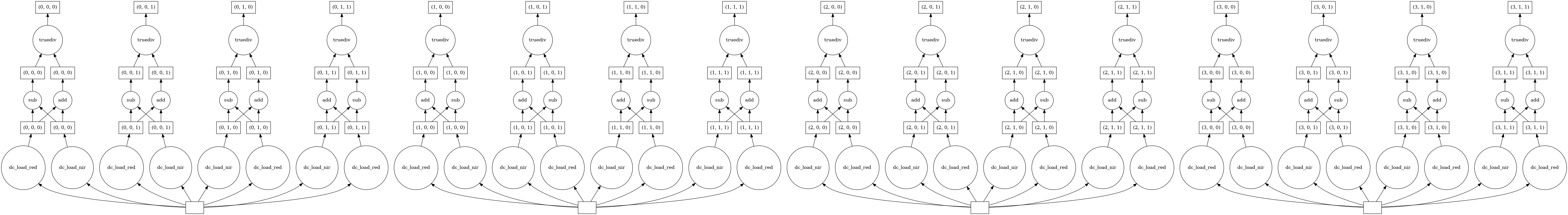
En visualisant le graphique de la tâche, nous pouvons maintenant voir l’équation NDVI se dérouler sur les quatre pas de temps de notre période de deux ans. Chaque pas de temps est indiqué par une entrée de base de données distincte au bas du graphique de la tâche (voir le pas de temps unique mis en évidence ci-dessous).

Affichage du tableau de bord pendant le calcul

Assurez-vous que votre nouvelle fenêtre avec le tableau de bord Dask est visible et exécutez la cellule suivante :

lazy_data_ndvi_compute = lazy_data.ndvi.compute()
lazy_data_ndvi_compute

<xarray.DataArray 'ndvi' (time: 4, y: 3317, x: 2895)>
array([[[0.06942078, 0.07080692, 0.0696223 , ..., 0.08328466,
         0.08114312, 0.08132118],
        [0.06951645, 0.0696682 , 0.06692324, ..., 0.08635357,
         0.0831899 , 0.07955576],
        [0.06737811, 0.06848731, 0.06940029, ..., 0.08616674,
         0.08235834, 0.07685342],
        ...,
        [0.38583474, 0.43568613, 0.4921664 , ..., 0.1825495 ,
         0.18272629, 0.18238801],
        [0.30237789, 0.37975794, 0.45614666, ..., 0.18378126,
         0.18577805, 0.18638376],
        [0.20758178, 0.28623428, 0.39149965, ..., 0.17947142,
         0.18378543, 0.18722567]],

       [[0.06175587, 0.06195676, 0.0608138 , ..., 0.07257672,
         0.07069745, 0.07147104],
        [0.06372657, 0.06219042, 0.05804492, ..., 0.07568556,
         0.07152239, 0.06959707],
        [0.06023316, 0.05772772, 0.05621204, ..., 0.07639401,
         0.07051051, 0.06657224],
...
        [0.50187138, 0.51266042, 0.54626763, ..., 0.09506223,
         0.09237813, 0.09149278],
        [0.3803492 , 0.46448664, 0.5345694 , ..., 0.09328612,
         0.09230149, 0.09234264],
        [0.2332595 , 0.35116818, 0.48972061, ..., 0.09416427,
         0.09450847, 0.0938633 ]],

       [[0.06011664, 0.06107649, 0.05899572, ..., 0.06922051,
         0.06808663, 0.06809524],
        [0.06101091, 0.06024636, 0.05826772, ..., 0.07232165,
         0.0690321 , 0.06698507],
        [0.05838208, 0.05756208, 0.06089405, ..., 0.07196642,
         0.06814041, 0.06525912],
        ...,
        [0.07636253, 0.07974138, 0.08053382, ..., 0.08965897,
         0.0869683 , 0.0873734 ],
        [0.07742436, 0.07760673, 0.07651878, ..., 0.08991228,
         0.08896701, 0.08775236],
        [0.07300672, 0.07317073, 0.07252679, ..., 0.09073517,
         0.09058855, 0.08816799]]])
Coordinates:
  * time         (time) datetime64[ns] 2020-03-31T23:59:59.999999 ... 2021-09...
  * y            (y) float64 3.702e+06 3.702e+06 ... 3.669e+06 3.669e+06
  * x            (x) float64 2.909e+06 2.909e+06 ... 2.938e+06 2.938e+06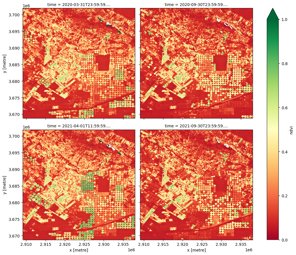
    spatial_ref  int32 6933

xarray.DataArray

'ndvi'

• time: 4
• y: 3317
• x: 2895

• 0.06942 0.07081 0.06962 0.06809 ... 0.08942 0.09074 0.09059 0.08817

  array([[[0.06942078, 0.07080692, 0.0696223 , ..., 0.08328466,
           0.08114312, 0.08132118],
          [0.06951645, 0.0696682 , 0.06692324, ..., 0.08635357,
           0.0831899 , 0.07955576],
          [0.06737811, 0.06848731, 0.06940029, ..., 0.08616674,
           0.08235834, 0.07685342],
          ...,
          [0.38583474, 0.43568613, 0.4921664 , ..., 0.1825495 ,
           0.18272629, 0.18238801],
          [0.30237789, 0.37975794, 0.45614666, ..., 0.18378126,
           0.18577805, 0.18638376],
          [0.20758178, 0.28623428, 0.39149965, ..., 0.17947142,
           0.18378543, 0.18722567]],
  
         [[0.06175587, 0.06195676, 0.0608138 , ..., 0.07257672,
           0.07069745, 0.07147104],
          [0.06372657, 0.06219042, 0.05804492, ..., 0.07568556,
           0.07152239, 0.06959707],
          [0.06023316, 0.05772772, 0.05621204, ..., 0.07639401,
           0.07051051, 0.06657224],
  ...
          [0.50187138, 0.51266042, 0.54626763, ..., 0.09506223,
           0.09237813, 0.09149278],
          [0.3803492 , 0.46448664, 0.5345694 , ..., 0.09328612,
           0.09230149, 0.09234264],
          [0.2332595 , 0.35116818, 0.48972061, ..., 0.09416427,
           0.09450847, 0.0938633 ]],
  
         [[0.06011664, 0.06107649, 0.05899572, ..., 0.06922051,
           0.06808663, 0.06809524],
          [0.06101091, 0.06024636, 0.05826772, ..., 0.07232165,
           0.0690321 , 0.06698507],
          [0.05838208, 0.05756208, 0.06089405, ..., 0.07196642,
           0.06814041, 0.06525912],
          ...,
          [0.07636253, 0.07974138, 0.08053382, ..., 0.08965897,
           0.0869683 , 0.0873734 ],
          [0.07742436, 0.07760673, 0.07651878, ..., 0.08991228,
           0.08896701, 0.08775236],
          [0.07300672, 0.07317073, 0.07252679, ..., 0.09073517,
           0.09058855, 0.08816799]]])

• Coordinates: (4)
  • time
    (time)
    datetime64[ns]
    2020-03-31T23:59:59.999999 ... 2...

    units :

    seconds since 1970-01-01 00:00:00

    array(['2020-03-31T23:59:59.999999000', '2020-09-30T23:59:59.999999000',
           '2021-04-01T11:59:59.999999000', '2021-09-30T23:59:59.999999000'],
          dtype='datetime64[ns]')

  • y
    (y)
    float64
    3.702e+06 3.702e+06 ... 3.669e+06

    units :

    metre

    resolution :

    -10.0

    crs :

    EPSG:6933

    array([3701915., 3701905., 3701895., ..., 3668775., 3668765., 3668755.])

  • x
    (x)
    float64
    2.909e+06 2.909e+06 ... 2.938e+06

    units :

    metre

    resolution :

    10.0

    crs :

    EPSG:6933

    array([2909105., 2909115., 2909125., ..., 2938025., 2938035., 2938045.])

  • spatial_ref
    ()
    int32
    6933

    spatial_ref :

    PROJCS["WGS 84 / NSIDC EASE-Grid 2.0 Global",GEOGCS["WGS 84",DATUM["WGS_1984",SPHEROID["WGS 84",6378137,298.257223563,AUTHORITY["EPSG","7030"]],AUTHORITY["EPSG","6326"]],PRIMEM["Greenwich",0,AUTHORITY["EPSG","8901"]],UNIT["degree",0.0174532925199433,AUTHORITY["EPSG","9122"]],AUTHORITY["EPSG","4326"]],PROJECTION["Cylindrical_Equal_Area"],PARAMETER["standard_parallel_1",30],PARAMETER["central_meridian",0],PARAMETER["false_easting",0],PARAMETER["false_northing",0],UNIT["metre",1,AUTHORITY["EPSG","9001"]],AXIS["Easting",EAST],AXIS["Northing",NORTH],AUTHORITY["EPSG","6933"]]

    grid_mapping_name :

    lambert_cylindrical_equal_area

    array(6933, dtype=int32)

• Attributes: (0)

Tracé de la série temporelle NDVI

lazy_data_ndvi_compute.plot(col='time', col_wrap= 2, cmap='RdYlGn',figsize=(11, 9),vmin=0, vmax=1)

<xarray.plot.facetgrid.FacetGrid at 0x7f4d38c3d880>

Concepts clés

• La fonction « create_local_dask_cluster() » tire parti de plusieurs cœurs de processeur pour accélérer les calculs, connus sous le nom de calcul distribué

• Le tableau de bord Dask nous permet de visualiser la progression des calculs au fur et à mesure de leur exécution en temps réel

Informations complémentaires

Client Dask

Dask peut utiliser plusieurs cœurs de calcul (CPU) en parallèle pour accélérer les calculs, ce que l’on appelle le calcul distribué.

Le package deafrica_tools nous donne accès aux fonctions de support au sein du module Dask, y compris la fonction create_local_dask_cluster(), qui nous permet de profiter des multiples processeurs disponibles dans le Sandbox.

Tableau de bord Dask

L’onglet d’état du planificateur fournit des informations sur les éléments suivants :

• Octets stockés : mémoire du cluster et mémoire par travailleur

• Traitement des tâches : tâches traitées par chaque travailleur

• Flux de tâches : affiche la progression de chaque tâche individuelle sur chaque thread, chaque ligne correspondant à un thread. Chaque couleur correspond à un type d’opération.

• Progrès : progression des calculs individuels

L’image ci-dessous montre le flux de tâches et la barre de progression au fur et à mesure de l’exécution des calculs.