Chargement différé des données
Par défaut, la bibliothèque « datacube » n’utilise pas Dask lors du chargement des données, ce qui signifie que lorsque « dc.load() » est utilisé, les données interrogées seront chargées en mémoire. Le chargement différé des données fait référence au chargement des données en mémoire uniquement lorsque cela est nécessaire à l’analyse. Afin de charger les données de manière différée, nous passons le paramètre « dask_chunks » dans l’instruction « dc.load() ».
Dans cette section, nous allons charger les données de manière différée en passant le paramètre « dask_chunks » dans la fonction « .load() » et explorer la structure des données des données chargées de manière différée.
Charger des paquets
[1]:
import datacube
import matplotlib.pyplot as plt
from deafrica_tools.dask import create_local_dask_cluster
from deafrica_tools.plotting import rgb, display_map
/usr/local/lib/python3.8/dist-packages/geopandas/_compat.py:112: UserWarning: The Shapely GEOS version (3.8.0-CAPI-1.13.1 ) is incompatible with the GEOS version PyGEOS was compiled with (3.10.3-CAPI-1.16.1). Conversions between both will be slow.
  warnings.warn(
Connexion au datacube
[2]:
dc = datacube.Datacube(app='Step1')
Fonction de charge standard
La commande « dc.load() » spécifie le produit, les mesures (bandes), les coordonnées x, y et la plage de temps.
[3]:
data = dc.load(product='gm_s2_annual',
              measurements=['red','green', 'blue', 'nir'],
              x=(31.90, 32.00),
              y=(30.49, 30.40),
              time=('2020-01-01', '2020-12-31'))

data
[3]:
<xarray.Dataset>
Dimensions:      (time: 1, y: 994, x: 965)
Coordinates:
  * time         (time) datetime64[ns] 2020-07-01T23:59:59.999999
  * y            (y) float64 3.713e+06 3.713e+06 ... 3.703e+06 3.703e+06
  * x            (x) float64 3.078e+06 3.078e+06 ... 3.088e+06 3.088e+06
    spatial_ref  int32 6933
Data variables:
    red          (time, y, x) uint16 2863 2892 3069 3104 ... 3367 3386 3425 3414
    green        (time, y, x) uint16 2222 2274 2403 2390 ... 2544 2555 2591 2589
    blue         (time, y, x) uint16 1514 1554 1644 1618 ... 1708 1706 1726 1732
    nir          (time, y, x) uint16 3832 3873 4010 3999 ... 3862 3893 3952 3937
Attributes:
    crs:           EPSG:6933
grid_mapping: spatial_refChargement paresseux des mêmes données
Le passage de « dask_chunks » dans la requête de chargement initialise le chargement paresseux des données, par lequel les objets « dask.array » sont renvoyés à la place des valeurs individuelles jusqu’à ce qu’ils soient appelés.
[4]:
# lazy loading data through dask chunks parameter
lazy_data = dc.load(product='gm_s2_annual',
                   measurements=['red','green', 'blue', 'nir'],
                   x=(31.90, 32.00),
                   y=(30.49, 30.40),
                   time=('2020-01-01', '2020-12-31'),
                   dask_chunks={'time':1,'x':500, 'y':500})
# return data
lazy_data
[4]:
<xarray.Dataset>
Dimensions:      (time: 1, y: 994, x: 965)
Coordinates:
  * time         (time) datetime64[ns] 2020-07-01T23:59:59.999999
  * y            (y) float64 3.713e+06 3.713e+06 ... 3.703e+06 3.703e+06
  * x            (x) float64 3.078e+06 3.078e+06 ... 3.088e+06 3.088e+06
    spatial_ref  int32 6933
Data variables:
    red          (time, y, x) uint16 dask.array<chunksize=(1, 500, 500), meta=np.ndarray>
    green        (time, y, x) uint16 dask.array<chunksize=(1, 500, 500), meta=np.ndarray>
    blue         (time, y, x) uint16 dask.array<chunksize=(1, 500, 500), meta=np.ndarray>
    nir          (time, y, x) uint16 dask.array<chunksize=(1, 500, 500), meta=np.ndarray>
Attributes:
    crs:           EPSG:6933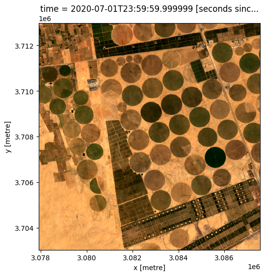
grid_mapping: spatial_refTracé d’une image RVB de la zone d’étude
[5]:
# View a rgb (true colour) image of study area
rgb(lazy_data, bands=['red', 'green', 'blue'])
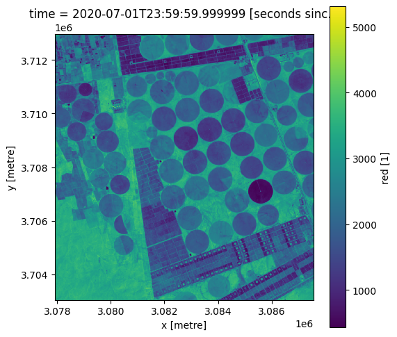
[6]:
# formatting the figure
fig , axis = plt.subplots(1, 1, figsize=(6, 6))
axis.set_aspect('equal')

lazy_data.red.plot(ax= axis)
[6]:
<matplotlib.collections.QuadMesh at 0x7f276c0c1a60>
Dans cette section, vous avez « chargé paresseusement » les données en passant le paramètre « dask_chunks » dans l’instruction de chargement.
Concepts clés
Jusqu’à présent, la fonction
.load()a été utilisée pour charger des données directement en mémoireDask est un outil utilisé pour diviser les données en morceaux gérables, idéal pour la gestion des données
L’ajout du paramètre « dask_chunks » à la fonction standard « .load() » nécessite que les données soient chargées paresseusement
Le chargement différé entraîne le chargement des données uniquement lorsque cela est nécessaire pour terminer un calcul, jusqu’à ce que des données spécifiques soient requises, le xarray.dataset est composé d’objets dask.array qui agissent comme des espaces réservés, et non comme des valeurs spécifiques
Pour diviser un ensemble de données en morceaux à l’aide de Dask, nous passons « dask_chunks » dans la requête de chargement et spécifions les paramètres « time », « x » et « y » (par exemple, « dask_chunks = {“time”: 1, “x”: 500, “y”: 500}``)
Informations complémentaires
Dask est un outil utilisé pour la gestion des données, ce processus décompose les données en blocs gérables stockés en mémoire. En bref, Dask vous permet de
analyser des ensembles de données plus grands que la mémoire
exécuter efficacement les calculs
Les opérations compatibles Dask ne sont pas exécutées tant que le calcul ou la visualisation des résultats finaux n’est pas demandé.
Charge standard
Dans cette section, nous avons utilisé la fonction standard « dc.load() » pour charger les données directement en mémoire. Jusqu’à présent, nous avons utilisé cette méthode de chargement des données du Datacube dans les notebooks Jupyter. Cependant, le chargement de données sur de grandes zones ou sur des périodes prolongées peut entraîner le blocage des notebooks Jupyter. Pour charger des ensembles de données plus volumineux, nous pouvons utiliser les fonctionnalités de Dask pour gérer le calcul dans une limite de mémoire limitée.
Chargement différé des données
Le chargement différé des données consiste à charger des données uniquement lorsqu’il est nécessaire de terminer un calcul. Pour charger des données de manière différée, nous ajoutons le paramètre « dask_chunks = {‘time’:, ‘x’:, ‘y’:} » dans l’instruction « dc.load() ». Lorsque nous chargeons de manière différée un ensemble de données, le « xarray.dataset » renvoyé est composé d’objets « dask.array ».
Le chargement différé des données permet d’économiser du temps et de la mémoire qui seraient autrement consacrés au stockage des données dans la mémoire locale de votre ordinateur.
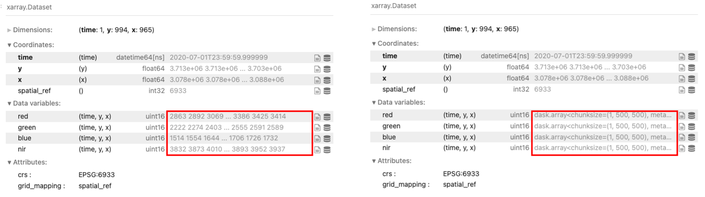
Remarque : la commande « .load() » avec le paramètre « dask_chunks » est beaucoup plus rapide car elle ne charge aucune donnée en mémoire. La comparaison ci-dessous montre les données renvoyées à l’aide de la fonction de chargement standard, puis les objets « dask.array » renvoyés lors du chargement différé du même « data.datacube ».
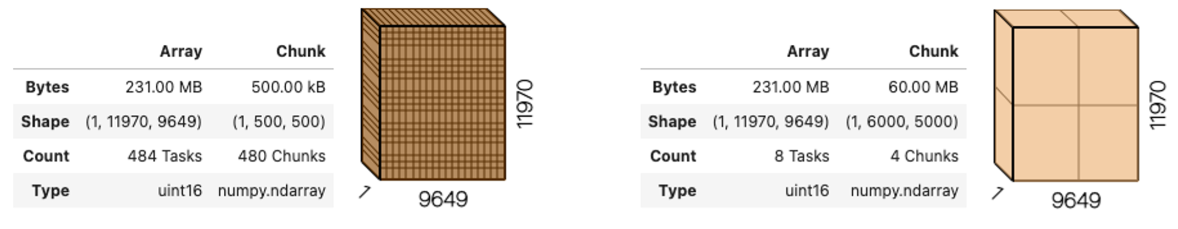
Factorisation de la forme du tableau Dask pour la segmentation
Lors du découpage des données, nous devons prendre en compte la forme des données, le type de calcul et la mémoire disponible. Vous trouverez ci-dessous un exemple montrant un nombre excessif de blocs contenant de petites quantités de données (480 blocs, chaque bloc stockant 500 kilo-octets de données). L’application des mêmes paramètres de découpage que précédemment dans cet exercice (x : 500, y : 500) est inefficace pour l’ensemble de données. Le découpage des données et la prise en compte de la taille des blocs, qui peuvent réduire le nombre de fois où les données doivent être lues à partir du fichier (moins de tâches et de blocs), sont plus efficaces en termes de temps.
Explication avancée
Plus grand que la mémoire fait référence aux ensembles de données qui nécessitent plus de stockage que la mémoire disponible, par exemple :
Exemple : pour charger trois bandes (rouge, vert, bleu), le type de données de chaque bande sera stocké sous forme d’entier non signé (uint16). Cela signifie que chaque pixel que vous souhaitez charger est de 16 bits, ce qui équivaut à 2 octets. Pour charger une zone de 100 pixels sur 100 pixels, vous devrez charger 10 000 pixels par bande, ce qui pour trois bandes nécessitera le chargement de 30 000 pixels. À 2 octets par pixel, cela représente un total de 60 000 octets (60 kilo-octets ou 0,06 gigaoctet). Cet exemple nécessite une petite quantité de mémoire qui s’intègre facilement dans la mémoire disponible dans votre Sandbox. Cependant, si vous souhaitez charger 12 bandes sur une zone plus grande couvrant 100 000 pixels par 100 000 pixels (10 000 km par 10 000 km pour une résolution Sentinel-2 de 10 m), cela nécessiterait 240 gigaoctets (100 000 pixels x 100 000 pixels x 12 bandes x 2 octets = 240 gigaoctets). Comme l’environnement Sandbox par défaut offre 16 Go de mémoire, cet ensemble de données hypothétique nécessiterait un stockage supplémentaire au-delà de ce qui est disponible et serait donc considéré comme plus grand que la mémoire.