Vectoriser et analyser les plans d’eau au Kenya

Produits utilisés : wofs_ls_summary_annual

Mots-clés données utilisées ; wofs_ls_summary_annual

Aperçu

Ce carnet détecte les plans d’eau dans une zone donnée en fonction d’un seuil de % d’observations d’eau. Il vectorise ensuite ces plans d’eau et exporte les résultats sous forme de fichier de formes. Cela peut être utilisé pour inspecter et étudier les plans d’eau d’une zone. Enfin, une série chronologique de la fréquence moyenne (% du temps) d’observation de l’eau au fil des années est affichée pour un plan d’eau sélectionné.

Description

Définir les paramètres pour la détection des plans d’eau.
Chargez la zone d’intérêt : une région du Kenya.
Charger WOfS pour la région.
Vectoriser et exporter des plans d’eau vers shapefile.
Inspectez un plan d’eau spécifique et tracez une série chronologique.

Commencer

Pour exécuter cette analyse, exécutez toutes les cellules du bloc-notes, en commençant par la cellule « Charger les packages ».

Charger des paquets

Importez les packages Python utilisés pour l’analyse.

[1]:

%matplotlib inline

from pathlib import Path

import rasterio.features
from shapely.geometry import Polygon, shape, mapping, MultiPolygon
from shapely.ops import unary_union
from odc.geo.geom import Geometry
from odc.geo.crs import CRS
import geopandas as gpd
import fiona
from fiona.crs import from_epsg
import xarray as xr
import pandas as pd
import glob
import os.path
import math
import geohash as gh
import re
import datacube
import seaborn as sns
import rioxarray
import matplotlib.pyplot as plt
import numpy as np

from deafrica_tools.spatial import xr_vectorize, xr_rasterize
from deafrica_tools.datahandling import wofs_fuser, mostcommon_crs
from deafrica_tools.plotting import map_shapefile

Se connecter au datacube

Connectez-vous au datacube pour que nous puissions accéder aux données de DE Africa.

[2]:

dc = datacube.Datacube(app='vectorise_waterbodies')

Seuil de détection des plans d’eau

Créez une valeur « minimum_wet_percentage » correspondant à la proportion de comptages humides au-dessus de laquelle une zone sera classée comme plan d’eau. Ce pourcentage fait référence au temps, c’est-à-dire au pourcentage de temps pendant lequel un pixel est mouillé. Il sera appliqué à la fréquence moyenne (%) calculée sur les années 2000 à 2021.

[3]:

minimum_wet_percentage = [0.25]

Nous définissons maintenant la plage de surface (m2) dans laquelle nous souhaitons que les plans d’eau se situent. Nous utiliserons les valeurs pour filtrer les plans d’eau détectés.

[4]:

min_area_m2 = 10000
max_area_m2 = 1500000

Nous pouvons également définir un seuil pour les observations valides minimales dont nous avons besoin pour déterminer que les observations humides sont des plans d’eau. Là encore, ce seuil sera appliqué au nombre moyen d’observations claires, « count_clear », calculé sur la période 2000 à 2021. La valeur par défaut est une moyenne de 5 observations valides par an.

[5]:

min_valid_observations = 5

apply_min_valid_observations_first = True

Charger et tracer la zone d’intérêt

Nous avons un fichier geojson qui définit un polygone pour la zone d’intérêt pour cette analyse. Nous pouvons voir le nom du comté et d’autres détails ci-dessous. Nous pouvons ensuite tracer les limites de la zone et cartographier le shapefile pour voir la zone sur laquelle nous travaillons.

[6]:

area = gpd.read_file('data/ccy.geojson').to_crs("epsg:6933")
area

[6]:

	County	ConsrvName	AreaHa	iddddd	geometry
0	Isiolo	Naapu	28143.325296731	1	MULTIPOLYGON (((3688221.493 188693.113, 368780...

[7]:

geom = Geometry(geom=area.iloc[0].geometry, crs="epsg:6933")

[8]:

map_shapefile(area, attribute = area.columns[0])

Configurer le répertoire d’exportation

Nous devons créer un dossier dans lequel exporter les résultats de notre fichier de formes. Nous allons créer un nom de fichier de base auquel nous pourrons faire référence lors de l’écriture de fichiers et stocker un objet de chemin de fichier dans le dossier d’exportation.

[9]:

base_filename = 'waterbodies'

intermediate_wb_path = Path('_wb_outputs/')

La cellule ci-dessous efface le répertoire d’exportation s’il existe déjà, puis crée un nouveau répertoire pour stocker les sorties du plan d’eau.

[10]:

%%bash
rm -rf _wb_outputs
mkdir _wb_outputs

Générer une requête et charger WOfS

Définissez la requête que nous utiliserons pour charger les données WOfS. Nous utiliserons la période 2000 à 2021, notre analyse est donc basée sur une période récente.

[11]:

resolution = (-30, 30)# This is the resolution of WOfS, which changes depending on which collection you use.
time_range = ('2000-01-01', '2021-12-31')

# how to chunk the dataset for use with dask
dask_chunks = {'x': 3000, 'y': 3000, 'time': 1}

Le « wofs_ls_summary_annual » fournit un résumé des observations de l’eau sur une base annuelle.

[12]:

query = {
    "geopolygon": geom,
    "resolution": resolution,
    "time": time_range,
    "dask_chunks": dask_chunks
}
output_crs = mostcommon_crs(dc=dc, product='wofs_ls_summary_annual', query=query)

# Then load the WOfS summary of clear/wet observations:
wofls = dc.load(product = 'wofs_ls_summary_annual', output_crs=output_crs,
               **query)


# And set the no-data values to nan:
wofls = wofls.where(wofls != -1)
print(wofls)

<xarray.Dataset> Size: 12GB
Dimensions:      (time: 22, y: 7651, x: 5756)
Coordinates:
  * time         (time) datetime64[ns] 176B 2000-07-01T23:59:59.999999 ... 20...
  * y            (y) float64 61kB 2.625e+05 2.625e+05 ... 3.308e+04 3.304e+04
  * x            (x) float64 46kB 3.556e+06 3.556e+06 ... 3.729e+06 3.729e+06
    spatial_ref  int32 4B 6933
Data variables:
    count_wet    (time, y, x) float32 4GB dask.array<chunksize=(1, 3000, 3000), meta=np.ndarray>
    count_clear  (time, y, x) float32 4GB dask.array<chunksize=(1, 3000, 3000), meta=np.ndarray>
    frequency    (time, y, x) float32 4GB dask.array<chunksize=(1, 3000, 3000), meta=np.ndarray>
Attributes:
    crs:           epsg:6933
    grid_mapping:  spatial_ref

Agrégat à moyenne sur la période d’intérêt

Calculez la moyenne annuelle de « count_wet », « count_clear » et « frequency » sur la période 2000 à 2021.

[13]:

wofls_lt = wofls.mean(dim='time')

Masquer la zone d’intérêt

[14]:

mask = xr_rasterize(area, wofls_lt)
wofls_lt = wofls_lt.where(mask) # select WOfS obersations within the area of interest

Vectoriser les polygones où la fréquence moyenne dépasse le seuil

Nous pouvons maintenant identifier les zones où la « fréquence » moyenne des observations humides dépasse le seuil (« minimum_wet_percentage ») et les convertir en polygones à l’aide de « xr_vectorize ». Les polygones qui se chevauchent sont fusionnés, puis enfin le fichier de formes de tous les plans d’eau détectés est exporté dans le répertoire que nous avons créé.

[15]:

# Filter pixels with at least the minimum valid observations.
wofs_valid_filtered = wofls_lt.count_clear >= min_valid_observations

# Remove any pixels that are wet less than the minimum wetness percentage of the time
wofs_filtered = wofls_lt.frequency > minimum_wet_percentage

# Now find pixels that meet both the minimum valid observations and wetness percentage criteria
# Change all zeros to NaN to create a nan/1 mask layer
# Pixels == 1 now represent our water bodies
if apply_min_valid_observations_first:
    wofs_filtered = wofs_filtered.where(wofs_filtered & wofs_valid_filtered)
else:
    wofs_filtered = wofs_filtered.where(wofs_filtered)

# Vectorise the raster.
polygons = xr_vectorize((wofs_filtered == 1), crs='EPSG:6933')
polygons = polygons[polygons.attribute == 1].reset_index(drop=True)

# Combine any overlapping polygons
polygons = polygons.geometry.buffer(0).union_all()

# Turn the combined multipolygon back into a geodataframe
polygons = gpd.GeoDataFrame(
geometry=list(polygons.geoms))
# We need to add the crs back onto the dataframe
polygons.crs = 'EPSG:6933'

# Calculate the area of each polygon again now that overlapping polygons
# have been merged
polygons['area'] = polygons.area

# Save the polygons to a shapefile
filename = intermediate_wb_path / f'{base_filename}_raw_{minimum_wet_percentage}.shp'
polygons.to_file(filename)

Combiner des polygones superposés en fonction des surfaces minimales et maximales

Nous allons maintenant utiliser les valeurs « min_area_m2 » et « max_area_m2 » que nous avons définies ci-dessus pour filtrer la collection de plans d’eau. Ce flux de travail a été conçu à l’origine pour des applications continentales, de sorte que certains aspects liés aux très grands polygones sont moins pertinents pour ce cas d’utilisation, bien que nous laisserons le code dans le flux de travail pour plus d’exhaustivité.

Le programme lit les plans d’eau que nous avons exportés dans le bloc-notes, puis filtre les plans d’eau qui dépassent ou sont inférieurs à nos seuils de superficie. Il identifie ensuite les petits plans d’eau qui sont inférieurs au seuil de superficie mais qui chevauchent d’autres plans d’eau, et les ajoute à l’ensemble de données final.

Les statistiques récapitulatives (superficie, périmètre et « Polsby-Popper <https://en.wikipedia.org/wiki/Polsby%E2%80%93Popper_test> ») sont ajoutées à l’ensemble de données avant qu’il ne soit à nouveau exporté et écrase les fichiers de formes précédents.

[16]:

polygons = gpd.read_file(filename)

threshold = minimum_wet_percentage[0]

assert minimum_wet_percentage[0] == max(minimum_wet_percentage)
polygons = gpd.read_file(filename)

# Filter polygons by size.
polygons = polygons[
    (polygons['area'] >= min_area_m2) & (polygons['area'] <= max_area_m2)]

# Combine detected polygons with their maximum extent boundaries.
lower_threshold = gpd.read_file(filename)
lower_threshold['area'] = pd.to_numeric(lower_threshold.area)

# Filter out those pesky huge polygons
lower_threshold = lower_threshold.loc[
    (lower_threshold['area'] <= max_area_m2)]
lower_threshold['lt_index'] = range(len(lower_threshold))

# Pull out the polygons from the extent shapefile that intersect with the detection shapefile
overlay_extent = gpd.overlay(polygons, lower_threshold, keep_geom_type=True)
lower_threshold_to_use = lower_threshold.loc[overlay_extent.lt_index]

# Combine the polygons
polygons = gpd.GeoDataFrame(
    pd.concat([lower_threshold_to_use, polygons], ignore_index=True))

# Merge overlapping polygons
polygons = polygons.union_all()

# Back into individual polygons
polygons = gpd.GeoDataFrame(crs='EPSG:6933', geometry=[polygons]).explode(index_parts=True)

# Get rid of the multiindex that explode added:
polygons = polygons.reset_index(drop=True)

# Add area, perimeter, and polsby-popper columns:
polygons['area'] = polygons.area
polygons['perimeter'] = polygons.length
polygons['pp_test'] = polygons.area * 4 * math.pi / polygons.perimeter ** 2

# Dump the merged polygons to a file:
polygons.to_file(f'_wb_outputs/{base_filename}_merged.shp')

Charger et inspecter les plans d’eau fusionnés

Nous pouvons maintenant charger les plans d’eau que nous avons stockés ci-dessus et inspecter les résultats. La cellule ci-dessous lit le fichier de formes que nous avons exporté et affiche les statistiques récapitulatives, la géométrie et la colonne d’identification que nous pouvons utiliser pour accéder à des plans d’eau spécifiques.

[17]:

waterbodies = gpd.read_file('_wb_outputs/waterbodies_merged.shp')
waterbodies['ID'] = waterbodies.index
waterbodies

[17]:

	area	perimeter	pp_test	geometry	ID
0	16200.0	600.0	0.565487	POLYGON ((3569100 65490, 3569070 65490, 356907...	0
1	56700.0	3540.0	0.056857	POLYGON ((3603840 79620, 3603840 79560, 360381...	1
2	38700.0	2340.0	0.088816	POLYGON ((3603240 81270, 3603240 81180, 360321...	2
3	11700.0	840.0	0.208371	POLYGON ((3602670 82530, 3602760 82530, 360276...	3
4	13500.0	960.0	0.184078	POLYGON ((3602190 82590, 3602190 82620, 360216...	4
...	...	...	...	...	...
57	20700.0	1320.0	0.149291	POLYGON ((3712500 110910, 3712500 110940, 3712...	57
58	14400.0	780.0	0.297429	POLYGON ((3713460 111690, 3713460 111720, 3713...	58
59	24300.0	1680.0	0.108193	POLYGON ((3717270 114510, 3717270 113700, 3717...	59
60	18900.0	1200.0	0.164934	POLYGON ((3717960 116430, 3717960 116460, 3718...	60
61	10800.0	660.0	0.311563	POLYGON ((3718680 116550, 3718680 116520, 3718...	61

62 rows × 5 columns

Nous pouvons tracer le shapefile pour visualiser les plans d’eau, ou nous pouvons explorer avec une carte de base satellite.

La cellule ci-dessous montre que la plupart des plans d’eau suivent un système fluvial.

[18]:

waterbodies.plot(edgecolor='k')

[18]:

<Axes: >

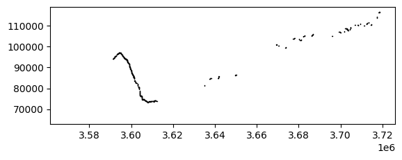
../../../../_images/sandbox_notebooks_Use_cases_surface_water_count_Vectorise_waterbodies_43_1.png

La cartographie du fichier de formes avec le code ci-dessous affiche les plans d’eau en bleu sur une carte de base satellite. Un zoom avant montre que l’analyse a capturé le système fluvial.

[19]:

map_shapefile(waterbodies, attribute = waterbodies.columns[0])

Sélectionnez un plan d’eau pour une analyse plus approfondie

Nous pouvons utiliser la fonction « .explore() » pour rechercher et sélectionner un plan d’eau pour une analyse plus approfondie. Bien que la plupart des plans d’eau suivent le système fluvial, nous pouvons voir qu’il existe un plan d’eau isolé à « 0,513, 36,989 ».

En inspectant la carte d’exploration ci-dessous, nous pouvons voir qu’il s’agit d’un plan d’eau avec ID = 0 et un périmètre de 600 m, situé près de Tura.

[20]:

waterbodies.explore()

[20]:

Make this Notebook Trusted to load map: File -> Trust Notebook

Analyse plus approfondie

Nous pouvons sélectionner le plan d’eau que nous avons identifié ci-dessus pour une analyse plus approfondie à l’aide de la sélection d’indices.

[21]:

geom = Geometry(geom=waterbodies.iloc[0].geometry, crs="epsg:6933")
geom

[21]:

../../../../_images/sandbox_notebooks_Use_cases_surface_water_count_Vectorise_waterbodies_49_0.svg

Nous pouvons masquer le résumé annuel du WOfS sur le polygone sélectionné.

[22]:

waterbody_ID = 0

geom = Geometry(waterbodies.iloc[waterbody_ID].geometry, crs='epsg:6933')

mask = rasterio.features.geometry_mask(
            [geom.to_crs(wofls.geobox.crs) for geoms in [geom]],
            out_shape=wofls.geobox.shape,
            transform=wofls.geobox.affine,
            all_touched=False,
            invert=True)
mask = xr.DataArray(mask, dims=("y", "x"))

wofl_masked = wofls.where(mask, drop=True)

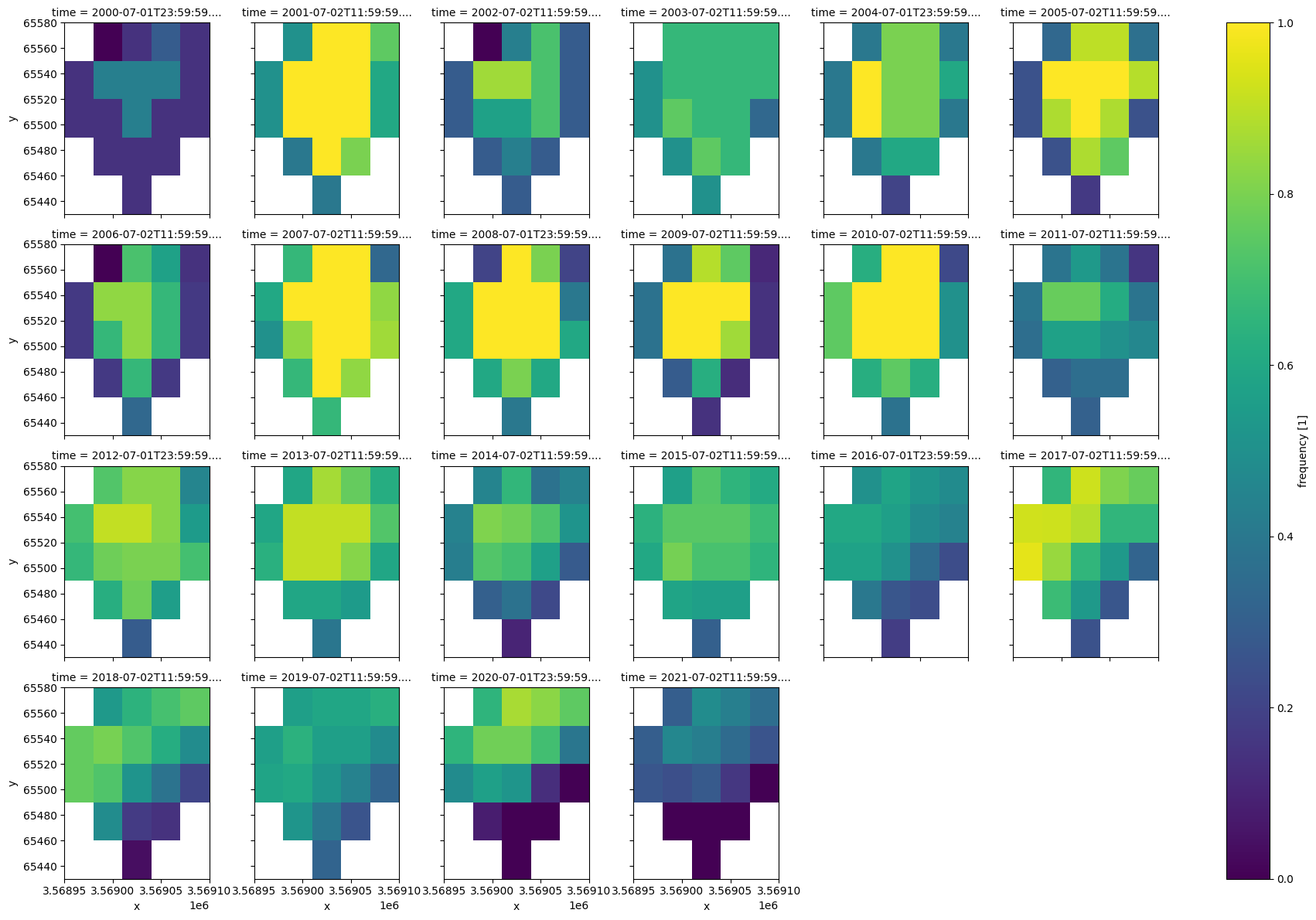
Nous pouvons inspecter la distribution de fréquence ; la proportion de fois dans chaque année où le pixel a été observé comme humide, sur chaque année pour notre plan d’eau sélectionné.

Cela montre que le milieu du plan d’eau a été constamment humide entre 2007 et 2010, mais la partie la plus humide du plan d’eau n’a été humide que pendant environ 60 à 70 % du temps en 2021.

[23]:

wofl_masked.frequency.isel().plot(col="time", col_wrap=6)

[23]:

<xarray.plot.facetgrid.FacetGrid at 0x7f9e623562d0>

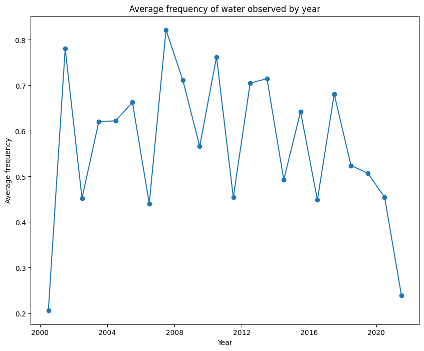
../../../../_images/sandbox_notebooks_Use_cases_surface_water_count_Vectorise_waterbodies_53_1.png

Enfin, nous pouvons réduire la dimension spatiale et tracer la fréquence moyenne indiquée ci-dessus sur une série chronologique.

[24]:

wofl_ts = wofl_masked.mean(['x','y'])

plt.figure(figsize = [10,8])
plt.plot(wofl_ts.time, wofl_ts.frequency, '-o')
plt.xlabel('Year')
plt.ylabel('Average frequency')
plt.title('Average frequency of water observed by year');

../../../../_images/sandbox_notebooks_Use_cases_surface_water_count_Vectorise_waterbodies_55_0.png

Informations Complémentaires

Licence : Le code de ce carnet est sous licence Apache, version 2.0 <https://www.apache.org/licenses/LICENSE-2.0>. Les données de Digital Earth Africa sont sous licence Creative Commons par attribution 4.0 <https://creativecommons.org/licenses/by/4.0/>.

Contact : Si vous avez besoin d’aide, veuillez poster une question sur le canal Slack Open Data Cube <http://slack.opendatacube.org/>`__ ou sur le GIS Stack Exchange en utilisant la balise open-data-cube (vous pouvez consulter les questions posées précédemment ici). Si vous souhaitez signaler un problème avec ce bloc-notes, vous pouvez en déposer un sur Github.

Version de Datacube compatible :

[25]:

print(datacube.__version__)

1.8.20

Dernier test :

[26]:

from datetime import datetime
datetime.today().strftime('%Y-%m-%d')

[26]:

'2025-01-17'