Prévision de l’étendue des eaux de surface dans le delta de l’Okavango

En utilisant les résultats de notre débit modélisé, des précipitations en amont et de la régression vectorielle automatique

Charger des paquets

Importez les packages Python utilisés pour l’analyse.

from statsmodels.tsa.vector_ar.var_model import VAR
from statsmodels.tsa.stattools import adfuller
from statsmodels.tools.eval_measures import rmse
from statsmodels.tsa.stattools import grangercausalitytests
import numpy as np
import pandas as pd
import matplotlib.pyplot as plt

Paramètres d’analyse

freq = 'Q-DEC'
data = 'results/okavango_all_datasets.csv'
modelled_discharge = 'results/modelled_discharge_Q-DEC.csv'

Lire les données

we=pd.read_csv(data, index_col='time', parse_dates=True)[['water_extent', 'okavango_rain']]
df=pd.read_csv(modelled_discharge, index_col=0, parse_dates=True)
df=df.join(we).drop(['water_discharge'],axis=1).dropna()
df.head(2)

	upstream_rainfall	predicted_discharge	water_extent	okavango_rain
2013-12-31	100.739380	11902.015733	52.2846	61.88324
2014-03-31	120.626221	27059.141065	163.8918	157.48248

Tester la causalité

La base de l’autorégression vectorielle est que chacune des séries temporelles du système s’influence mutuellement. Autrement dit, vous pouvez prédire la série avec ses valeurs passées ainsi que celles d’autres séries du système. Ci-dessous, nous effectuons un test de causalité de Granger pour voir si les variables sont liées les unes aux autres. Dans le tableau qui est imprimé après l’exécution des deux cellules ci-dessous, une valeur p donnée est < niveau de signification (0,05), puis la série X correspondante (colonne) provoque le Y (ligne).

# def grangers_causation_matrix(data, variables, maxlag=3, test='ssr_chi2test', verbose=False):
#     """Check Granger Causality of all possible combinations of the Time series.
#     The rows are the response variable, columns are predictors. The values in the table
#     are the P-Values. P-Values lesser than the significance level (0.05), implies
#     the Null Hypothesis that the coefficients of the corresponding past values is
#     zero, that is, the X does not cause Y can be rejected.

#     data      : pandas dataframe containing the time series variables
#     variables : list containing names of the time series variables.
#     """
#     df = pd.DataFrame(np.zeros((len(variables), len(variables))), columns=variables, index=variables)
#     for c in df.columns:
#         for r in df.index:
#             test_result = grangercausalitytests(data[[r, c]], maxlag=maxlag, verbose=False)
#             p_values = [round(test_result[i+1][0][test][1],4) for i in range(maxlag)]
#             if verbose: print(f'Y = {r}, X = {c}, P Values = {p_values}')
#             min_p_value = np.min(p_values)
#             df.loc[r, c] = min_p_value
#     df.columns = [var + '_x' for var in variables]
#     df.index = [var + '_y' for var in variables]
#     return df

# grangers_causation_matrix(df, variables = df.columns)

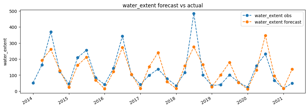
Effectuer des back-tests itératifs pour valider la capacité de prévision

Nous allons ici effectuer une prévision, mais sur un intervalle de la série temporelle pour lequel nous disposons déjà d’observations. Cela nous permettra de tester la capacité de prévision du modèle.

Commençons d’abord par initier un modèle

model=VAR(df, freq=freq)

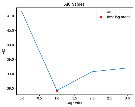
Trouver le meilleur ordre de décalage en utilisant le critère d’information d’Akaike (AIC)

#calculate AIC
x=model.select_order(maxlags=3)
aic=pd.read_html(x.summary().as_html(),header=0, index_col=0)[0][['AIC']]
aic['AIC']=[float(i[0:5]) for i in aic.values.flatten()]
lag_order = aic.idxmin().values[0]

#plot
aic.plot()
plt.scatter(lag_order, aic.loc[lag_order], color='r', label='best lag order')
plt.title('AIC Values')
plt.ylabel('AIC')
plt.xlabel('Lag Order')
plt.legend()
print("Lag order to use is "+str(lag_order))

Lag order to use is 1

Créer et adapter un modèle sur les données

En utilisant l’ordre de décalage défini ci-dessus

model=VAR(df, freq=freq)
model_fit = model.fit(1)

forecast_length = lag_order

n_windows = int((len(df) / forecast_length) - 1)
window_size = forecast_length

aa = window_size
dfs=[]
for i in range(0, n_windows):
    start=aa+lag_order
    end=(aa)
    backtest_input = df.values[-start:-end]
    fc = model_fit.forecast(y=backtest_input, steps=window_size)
    if i == 0:
        index=df.index[-end:]
    else:
        index=df.index[-end:-(end-window_size)]
    fc = pd.DataFrame(fc, index=index, columns=df.columns)
    dfs.append(fc)
    aa+=window_size

#concat results together
fc=pd.concat(dfs)
fc.columns = fc.columns.get_level_values(0)

test=df[df.index.isin(fc.index)]
for i in test.columns:
    print('rmse value for', i, 'is : ', round(rmse(fc[[i]], test[[i]])[0],2))

rmse value for upstream_rainfall is :  48.79
rmse value for predicted_discharge is :  15682.77
rmse value for water_extent is :  183.53
rmse value for okavango_rain is :  44.29

col = 'water_extent'
plt.figure(figsize=(12,4))
plt.plot(df.index, df[col], label=col+' obs',linestyle='dashed', marker='o')
fc[col].plot(label=col+' forecast',linestyle='dashed', marker='o')
plt.ylabel(col)
plt.title(col+" forecast vs actual")
plt.legend();

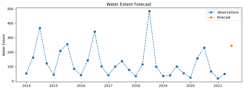
Prévision de l’étendue de l’eau

#make final predictions
model = VAR(endog=df, freq=freq)
model_fit = model.fit(lag_order)

pred = model_fit.forecast(df.values[-model_fit.k_ar:], steps=forecast_length)

#converting predictions to dataframe
cols = df.columns
fc = pd.DataFrame(index=range(0,len(pred)), columns=[cols])
for j in range(0,len(cols)):
    for i in range(0, len(pred)):
        fc.iloc[i][j] = pred[i][j]

fc.index = pd.date_range(freq=freq, start=df.index[-1], periods=len(fc)+1)[1:]
fc.head()

	upstream_rainfall	predicted_discharge	water_extent	okavango_rain
2021-06-30	-12.659938	34071.346128	244.632889	-7.007658

plt.figure(figsize=(12,4))
plt.plot(df.index, df['water_extent'], label='observations',linestyle='dashed', marker='o')
plt.plot(fc.index, fc[['water_extent']], label='forecast',linestyle='dashed', marker='o')
plt.ylabel('Water Extent')
plt.title("Water Extent Forecast")
# plt.ylim(0.0,0.9)
plt.legend();

---

Informations Complémentaires

Licence : Le code de ce carnet est sous licence Apache, version 2.0 <https://www.apache.org/licenses/LICENSE-2.0>. Les données de Digital Earth Africa sont sous licence Creative Commons par attribution 4.0 <https://creativecommons.org/licenses/by/4.0/>.

Contact : Si vous avez besoin d’aide, veuillez poster une question sur le canal Slack Open Data Cube <http://slack.opendatacube.org/>`__ ou sur le GIS Stack Exchange en utilisant la balise open-data-cube (vous pouvez consulter les questions posées précédemment ici). Si vous souhaitez signaler un problème avec ce bloc-notes, vous pouvez en déposer un sur Github.

Dernier test :

from datetime import datetime
datetime.today().strftime('%Y-%m-%d')

'2023-08-21'