Surveillance des zones humides dans l’Okavango

Produits utilisés : ls8_sr, wofs_ls, fc_ls

Aperçu

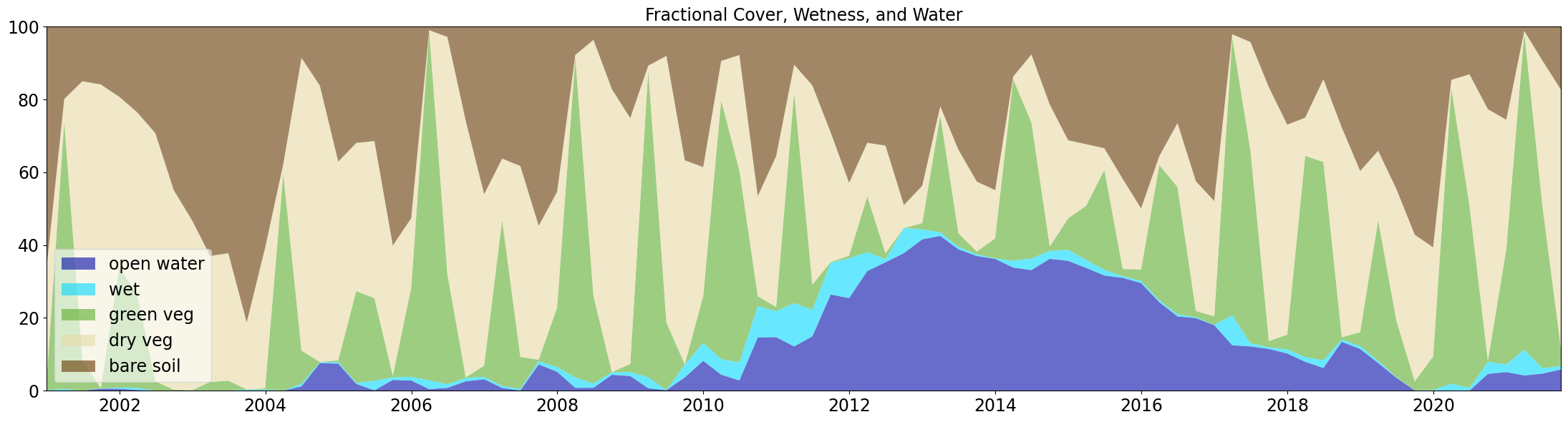
L’outil « Wetlands Insight Tool (WIT) » fournit des informations sur la dynamique saisonnière et interannuelle d’une zone humide. Le WIT est un résumé spatiotemporel d’une zone humide qui combine plusieurs ensembles de données dérivés des archives Landsat conservées au sein de DE Africa. Les données « Couverture fractionnaire », « WOfS » et « Réflectance de surface Landsat » sont extraites de l’ODC de DE Africa et combinées pour produire un graphique de pile décrivant le pourcentage d’un polygone de zone humide en termes de couverture fractionnaire de végétation, d’eau libre et de végétation humide au fil du temps.

Explication détaillée : Le code calcule l’humidité du capuchon à pompons (TCW, ou simplement « humidité ») à partir de la réflectance de surface et prend la fraction de couverture fractionnaire maximale par pixel, en masquant la couverture fractionnaire avec TCW et en masquant TCW avec de l’eau libre. Pour chaque pixel à l’intérieur ou chevauchant le polygone décrivant la zone humide, WIT calcule le type de couverture fractionnaire dominant. WIT sélectionne la valeur de pourcentage la plus élevée pour chaque pixel comme type de couverture fractionnaire dominant. La couverture fractionnaire a été masquée à l’aide de WOfS et TCW pour supprimer les zones d’eau et de végétation humide des zones où la couverture fractionnaire est calculée. Cela est nécessaire car l’algorithme de couverture fractionnaire classe par erreur l’eau comme végétation verte (PV). Le résultat obtenu est un graphique empilé d’eau libre, de végétation humide, de végétation photosynthétique, de végétation non photosynthétique et de sol nu pour le polygone de zone humide au fil du temps.

Description

Ce bloc-notes exécutera l’outil Wetlands Insight pour la zone englobée par un polygone

Charger dans un shapefile
Exécutez l’outil Wetlands Insight
Tracez les résultats sous forme de graphique à lignes empilées

Commencer

Pour exécuter cette analyse, exécutez toutes les cellules du bloc-notes, en commençant par la cellule « Charger les packages ». ***

Charger des paquets

[1]:

import datacube
import pandas as pd
import seaborn as sns
import geopandas as gpd
import matplotlib.pyplot as plt
from odc.geo.geom import geometry

from deafrica_tools.wetlands import WIT_drill

from deafrica_tools.datahandling import load_ard
from deafrica_tools.plotting import map_shapefile
from deafrica_tools.dask import create_local_dask_cluster

[2]:

create_local_dask_cluster()

/opt/venv/lib/python3.12/site-packages/distributed/node.py:187: UserWarning: Port 8787 is already in use.
Perhaps you already have a cluster running?
Hosting the HTTP server on port 35623 instead
  warnings.warn(

Client

Client-11bf5ed2-d4a2-11ef-8ba0-1ede66a139be

Connection method: Cluster object	Cluster type: distributed.LocalCluster
Dashboard: /user/victoria@kartoza.com/proxy/35623/status

Cluster Info

LocalCluster

779973fd

Dashboard: /user/victoria@kartoza.com/proxy/35623/status	Workers: 1
Total threads: 7	Total memory: 59.21 GiB
Status: running	Using processes: True

Scheduler Info

Scheduler

Scheduler-a6facb0e-9aec-456e-8ba6-62ecfd3a42de

Comm: tcp://127.0.0.1:44749	Workers: 1
Dashboard: /user/victoria@kartoza.com/proxy/35623/status	Total threads: 7
Started: Just now	Total memory: 59.21 GiB

Workers

Worker: 0

Comm: tcp://127.0.0.1:36155	Total threads: 7
Dashboard: /user/victoria@kartoza.com/proxy/36765/status	Memory: 59.21 GiB
Nanny: tcp://127.0.0.1:45499
Local directory: /tmp/dask-scratch-space/worker-7bxngwh9

Paramètres d’analyse

La cellule suivante définit des paramètres importants pour l’analyse :

shp_path : un chemin d’accès au fichier vectoriel (par exemple, folder/input.shp).
time_range : la plage de dates à analyser (par exemple ('2015', '2019'))

[3]:

shp_path = 'data/lake_ngami.geojson'

time_range = ('2000-12' , '2021-08')

Charger le fichier de formes

Nous nous assurerons également que le polygone est en coordonnées WGS84 (epsg=4326) en utilisant la méthode to_crs() pour nous assurer qu’il peut indexer correctement le datacube.

[4]:

gdf = gpd.read_file(shp_path).to_crs('epsg:4326')

Tracer le polygone

Cette cellule tracera le polygone sur une carte de base en utilisant la fonction deafrica_tools.plotting map_shapefile

[5]:

#plot the shapefile over a basemap
gdf['id']=0
map_shapefile(gdf, attribute='id', fillOpacity=0.1)

Exécutez l’outil Wetlands Insight

Même pour les petites zones, ce code peut prendre beaucoup de temps à exécuter, vous devrez donc être patient. En effet, l’outil charge trois ensembles de données distincts (Landsat SR, Fractional Cover et WOfS) et calcule un indice de cap à pompons à la volée.

Si la région est grande et/ou la durée est longue, la cellule ci-dessous prendra beaucoup de temps à s’exécuter. Utilisez le « Dask Dashboard » pour surveiller la progression.

[6]:

export_name='results/lake_ngami_WIT.csv'

[7]:

df = WIT_drill(
    gdf=gdf,
    time=time_range,
    min_gooddata=0.0,
    TCW_threshold=-0.035,
    resample_frequency="Q-DEC",
    export_csv=export_name,
    dask_chunks=dict(x=1000, y=1000, time=1),
    verbose=False,
)

df.head()

/opt/venv/lib/python3.12/site-packages/rasterio/warp.py:387: NotGeoreferencedWarning: Dataset has no geotransform, gcps, or rpcs. The identity matrix will be returned.
  dest = _reproject(

[7]:

	wofs_area_percent	wet_percent	green_veg_percent	dry_veg_percent	bare_soil_percent
2000-12-31	0.00	0.11	1.14	31.66	67.09
2001-03-31	0.00	0.48	73.46	6.21	19.85
2001-06-30	0.00	0.00	8.48	76.54	14.98
2001-09-30	0.57	0.11	0.00	83.45	15.87
2001-12-31	0.53	0.31	33.02	46.90	19.23

Tracer les résultats

Si vous souhaitez exporter le tracé sous forme de fichier .png, définissez la variable ci-dessous sur « True » et donnez un « nom » au tracé (par exemple, le nom de la zone humide).

[8]:

export_plot = True
out_filename = 'results/Lake_Ngami_WIT.png'

[9]:

fontsize = 17

# generate plot

#set up color palette
pal = [sns.xkcd_rgb["cobalt blue"],
       sns.xkcd_rgb["neon blue"],
       sns.xkcd_rgb["grass"],
       sns.xkcd_rgb["beige"],
       sns.xkcd_rgb["brown"]]

#make a stacked area plot
plt.clf()
fig=plt.figure(figsize = (22,6))
plt.stackplot(df.index,
              df.wofs_area_percent,
              df.wet_percent,
              df.green_veg_percent,
              df.dry_veg_percent,
              df.bare_soil_percent,
              labels=['open water',
                      'wet',
                      'green veg',
                      'dry veg',
                      'bare soil',
                     ], colors=pal, alpha = 0.6)

#set axis limits to the min and max
plt.axis(xmin = df.index[0], xmax = df.index[-1], ymin = 0, ymax = 100)
plt.tick_params(labelsize=fontsize)
#add a legend and a tight plot box
plt.legend(loc='lower left', framealpha=0.6, fontsize=fontsize)
plt.title('Fractional Cover, Wetness, and Water', fontsize=fontsize)
plt.tight_layout();
if export_plot:
    #save the figure
    plt.savefig(out_filename);

<Figure size 640x480 with 0 Axes>

../../../../_images/sandbox_notebooks_Use_cases_Okavango_0_Wetland_inundation_and_vegetation_dynamics_16_1.png

Informations Complémentaires

Licence : Le code de ce carnet est sous licence Apache, version 2.0 <https://www.apache.org/licenses/LICENSE-2.0>. Les données de Digital Earth Africa sont sous licence Creative Commons par attribution 4.0 <https://creativecommons.org/licenses/by/4.0/>.

Contact : Si vous avez besoin d’aide, veuillez poster une question sur le canal Slack Open Data Cube <http://slack.opendatacube.org/>`__ ou sur le GIS Stack Exchange en utilisant la balise open-data-cube (vous pouvez consulter les questions posées précédemment ici). Si vous souhaitez signaler un problème avec ce bloc-notes, vous pouvez en déposer un sur Github.

Version compatible ``datacube`` :

[10]:

print(datacube.__version__)

1.8.20

Dernier test :

[11]:

from datetime import datetime
datetime.today().strftime('%Y-%m-%d')

[11]:

'2025-01-17'