
Service de surveillance de la qualité de l’eau (WQMS) de Digital Earth Africa#
Produits utilisés : wq_annual
Mots-clés qualité de l’eau, données utilisées ; wq_annual
Aperçu#
Ce notebook fait partie d’une collection de notebooks d’analyse de la qualité de l’eau qui utilisent des données d’observation de la Terre pour évaluer les conditions des eaux de surface. Ensemble, ces notebooks offrent une vision plus globale de la qualité de l’eau en permettant une analyse à travers de multiples indicateurs.
Ce notebook présente les différentes variables disponibles dans le produit de qualité de l’eau annuel. Des flux de travail sont fournis pour surveiller ces variables sur des échelles de temps plus courtes, comme pour la turbidité et l” indice des algues flottantes (Floating Algae Index).
Le Service de surveillance de la qualité de l’eau (WQMS) fournit des informations sur la qualité de l’eau des plans d’eau de surface à travers le continent africain. Les données d’observation de la Terre (EO) offrent une couverture spatiale continue et une surveillance des changements à une fraction du coût et de la complexité logistique de la surveillance in-situ. Alors que les gouvernements nationaux à travers l’Afrique travaillent pour répondre au sous-indicateur 2 de l” Objectif de développement durable (ODD) 6.6.1 — Qualité de l’eau des lacs et des plans d’eau artificiels — le Système de surveillance de la qualité de l’eau (WQMS) fournira des informations opportunes et pertinentes pour la prise de décision afin de soutenir la gestion et l’utilisation durable des ressources en eau de surface. Cela inclut des indicateurs tels que la turbidité globale de l’eau et l’indice d’état trophique, qui sert de substitut à la santé biologique d’un plan d’eau.
Description#
Ce notebook démontre comment charger les données annuelles de qualité de l’eau de DE Africa en utilisant le logiciel Open Data Cube. Les sujets abordés incluent :
Charger et inspecter les données annuelles de qualité de l’eau
Remarque : Consultez le Guide de l’utilisateur de la qualité de l’eau de DE Africa pour des informations techniques détaillées, notamment sur les méthodes, la qualité et l’accès aux données.
Commencer#
Pour exécuter cette analyse, exécutez toutes les cellules du bloc-notes, en commençant par la cellule « Charger les packages ».
Charger des paquets#
Importez les packages Python utilisés pour l’analyse.
[6]:
%matplotlib inline

import datacube
import numpy as np
import matplotlib.pyplot as plt
from matplotlib.colors import ListedColormap, BoundaryNorm
from matplotlib.gridspec import GridSpec
import cmocean  # For nice ocean colour maps
from deafrica_tools.plotting import display_map, xr_animation
from deafrica_tools.waterbodies import get_waterbody, get_water_quality_summary, get_water_quality_rankings
from IPython.core.display import Video
Se connecter au datacube#
Connectez-vous au datacube pour que nous puissions accéder aux données de DE Africa. Le paramètre « app » est un nom unique pour l’analyse qui est basé sur le nom du fichier du notebook.
[7]:
dc = datacube.Datacube(app="DE_Africa_Water_Quality_Monitoring_Service")
Charger et inspecter les données annuelles de qualité de l’eau#
Définissez l’emplacement (gamme lat/lon) et la période pour extraire les données de qualité de l’eau. L’emplacement par défaut est le lac Ichkeul dans le nord de la Tunisie.
Nous définissons explicitement la liste des couches de qualité de l’eau à charger.
[8]:
query = {
    "product": "wq_annual",
    "x": (9.56, 9.77),
    "y": (37.11, 37.21),
    "crs": "EPSG:4326",
    "time": ("2000-01-01", "2025-12-31"),
    "output_crs": "EPSG:6933",
    "resolution": (-10, 10),
    "measurements": [
        "tsm",  # Turbidity
        "chla",  # Chlorophyll-A
        "tsi",  # Trophic State Index
        "agm_ndvi",  # NDVI
        "agm_hue",  # Water Hue
        "agm_owt",  # Optical Water Type
        "agm_fai",  # Floating Algal Index
        "clear_water",  # Clear water mask
        "water_mask",  # Water presence mask
        "tirs_st_ann_max",  # Max water surface temperature
        "tirs_st_ann_med",  # Median water surface temperature
        "tirs_st_ann_min",  # Min water surface temperature
    ],
}
[9]:
display_map(x=query["x"], y=query["y"])
[9]:
[10]:
ds = dc.load(**query)
[11]:
ds
[11]:
<xarray.Dataset> Size: 3GB
Dimensions:          (time: 26, y: 1022, x: 2028)
Coordinates:
  * time             (time) datetime64[ns] 208B 2000-07-01T23:59:59.999999 .....
  * y                (y) float64 8kB 4.428e+06 4.427e+06 ... 4.417e+06 4.417e+06
  * x                (x) float64 16kB 9.224e+05 9.224e+05 ... 9.427e+05
    spatial_ref      int32 4B 6933
Data variables:
    tsm              (time, y, x) float32 216MB nan nan nan nan ... nan nan nan
    chla             (time, y, x) float32 216MB nan nan nan nan ... nan nan nan
    tsi              (time, y, x) float32 216MB nan nan nan nan ... nan nan nan
    agm_ndvi         (time, y, x) float32 216MB nan nan nan nan ... nan nan nan
    agm_hue          (time, y, x) float32 216MB nan nan nan nan ... nan nan nan
    agm_owt          (time, y, x) float32 216MB nan nan nan nan ... nan nan nan
    agm_fai          (time, y, x) float32 216MB nan nan nan nan ... nan nan nan
    clear_water      (time, y, x) float32 216MB nan nan nan nan ... nan nan nan
    water_mask       (time, y, x) float32 216MB nan nan nan nan ... nan nan nan
    tirs_st_ann_max  (time, y, x) float32 216MB nan nan nan nan ... nan nan nan
    tirs_st_ann_med  (time, y, x) float32 216MB nan nan nan nan ... nan nan nan
    tirs_st_ann_min  (time, y, x) float32 216MB nan nan nan nan ... nan nan nan
Attributes:
    crs:           EPSG:6933
grid_mapping: spatial_refMasques d’eau#
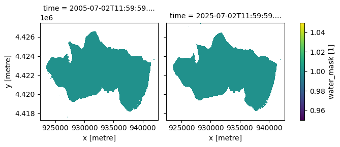
Comme on peut le voir ci-dessus, plusieurs variables sont disponibles. Ci-dessous, nous traçons le masque de présence d’eau, généré à partir du produit WOfS sur une période glissante de 5 ans (car la végétation flottante peut dominer la surface de l’eau pendant de longues périodes).
Pour les premières couches de qualité de l’eau ci-dessous, nous visualiserons des cartes de 2005 et 2025. Différentes années peuvent être sélectionnées pour différents plans d’eau.
[12]:
ds.sel(time=ds.time.dt.year.isin([2005, 2025])).water_mask.plot(col="time");
Indice d’algues flottantes (FAI)#
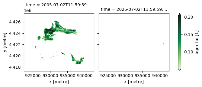
L’indice des algues flottantes (Floating Algae Index - FAI) est utilisé pour détecter et surveiller la végétation flottante et les efflorescences algales, qui sont souvent problématiques ou dangereuses. Le FAI soutient l’alerte précoce et la gestion des risques. Les zones d’algues et de végétation de surface doivent également être cartographiées avant d’appliquer les algorithmes pour la chlorophylle-A ou la turbidité. Le FAI n’est fourni que lorsqu’il est supérieur à un seuil de 0,05, c’est-à-dire lorsqu’il y a une présence probable d’algues flottantes.
[13]:
ds.agm_fai.sel(time=ds.time.dt.year.isin([2005, 2025])).plot(
    robust=True, col="time", cmap="cmo.algae"
);
Masque d’eau claire#
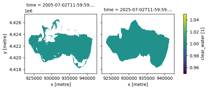
Le masque d’eau claire est défini comme les zones où l’eau est détectée et où le FAI est inférieur au seuil de 0,05. Les couches suivantes — y compris le type d’eau optique, la teinte (hue), les matières en suspension totales, la chlorophylle-a et l’indice d’état trophique — ne contiennent des valeurs qu’à l’intérieur du masque clear_water.
[14]:
ds.clear_water.sel(time=ds.time.dt.year.isin([2005, 2025])).plot(col="time");
Matières totales en suspension (MTS)#
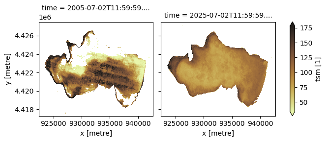
Les matières en suspension totales (TSM) annuelles sont fournies comme un indicateur sur une échelle relative, avec des valeurs conçues pour correspondre à \(\mathrm{mg}/\mathrm{m^3}\) de particules en suspension. Les valeurs TSM sont liées à la turbidité ou à l’opacité de l’eau. Des valeurs TSM plus élevées peuvent obstruer les habitats aquatiques et réduire la productivité de l’écosystème et la génération d’oxygène.
[15]:
ds.tsm.sel(time=ds.time.dt.year.isin([2005, 2025])).plot(
    robust=True, col="time", cmap="cmo.turbid"
);
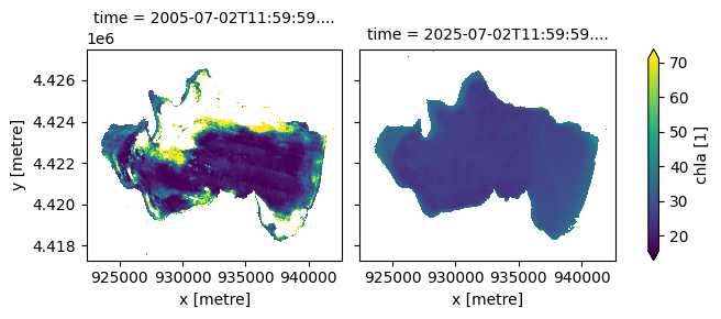
Chlorophylle-A (ChlA)#
Chlorophyll-A is an indicator of algal content, used to identify conditions conducive to algal blooms and assess biological productivity. ChlA is provided as an indicator on a relative scale, with values designed to correspond to \(\mathrm{mg}/\mathrm{m^3}\). ChlA is readily transformed to the Trophic State Index used in SDG reporting, as is done in the next cell.
[16]:
ds.chla.sel(time=ds.time.dt.year.isin([2005, 2025])).plot(robust=True, col="time");
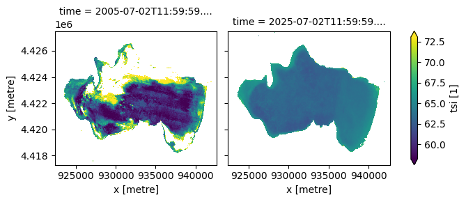
Trophic State Index (TSI)#
Derived from chlorophyll-a, the TSI provides an indicator of lake trophic status and productivity. Values typically range from 0 to 100, with higher values reflecting greater algal biomass and increasing eutrophication. In this product, the TSI is calculated as a logarithmic function of chlorophyll-a concentration, following Carlson 1977, with a continuous relationship fitted to the published ChlA–TSI class relationships to estimate TSI directly rather than using discrete class bins.
[17]:
ds.tsi.sel(time=ds.time.dt.year.isin([2005, 2025])).plot(robust=True, col="time");
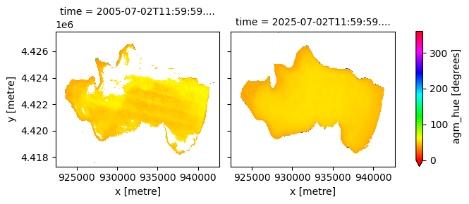
Hue#
The water colour, also known as the hue of the water, derived from the spectral reflectances measured by the EO instruments. Hue is expressed as an angle from 0-360. The hue of the waterbody is an objective way to determine changes in water colour.
[18]:
ds.agm_hue.sel(time=ds.time.dt.year.isin([2005, 2025])).plot(
    robust=True, col="time", cmap="hsv", vmin=0, vmax=360
);
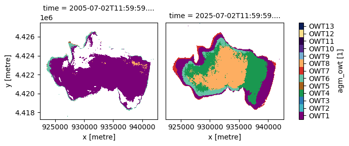
Optical Water Type (OWT)#
OWT (Spyrakos et al., 2018) is a classification of water types used to support EO based monitoring of water quality. For inland waters 13 OWTs are identified based on their spectral characteristics. These can then be characterised as oligotrophic, eutrophic, or hypereutrophic water types. The OWT of a waterbody may change seasonally or over the longer term.
OWT |
Class |
Dominant Characteristics |
|---|---|---|
OWT1 |
eutrophic_and_blue_green |
Hypereutrophic waters with scum of cyanobacterial bloom and vegetation-like Rrs |
OWT2 |
eutrophic_and_blue_green |
Common case waters with diverse reflectance shape and marginal dominance of pigments and Colored Dissolved Organic Matter (CDOM) over inorganic suspended particles |
OWT3 |
oligotrophic_clear |
Clear waters |
OWT4 |
eutrophic_and_blue_green |
Turbid waters with high organic content |
OWT5 |
eutrophic_and_blue_green |
Sediment-laden waters |
OWT6 |
hyper_eutrophic_green_brown |
Balanced effects of optically active constituents at shorter wavelengths |
OWT7 |
hyper_eutrophic_green_brown |
Highly productive waters with high cyanobacteria abundance and elevated reflectance at red/near-infrared spectral region |
OWT8 |
hyper_eutrophic_green_brown |
Productive waters with cyanobacteria presence and with remote sensing reflectance (Rrs) peak close to 700 nm |
OWT9 |
oligotrophic_clear |
Optically neighboring to OWT2 waters but with higher Rrs at shorter wavelengths |
OWT10 |
hyper_eutrophic_green_brown |
CDOM-rich waters |
OWT11 |
eutrophic_and_blue_green |
Waters high in CDOM with cyanobacteria presence and high absorption efficiency by Non-Algal Particles (NAP) |
OWT12 |
eutrophic_and_blue_green |
Turbid, moderately productive waters with cyanobacteria presence |
OWT13 |
oligotrophic_clear |
Very clear blue waters |
[19]:
# Same colours as DE Africa Maps
colors = [
    "#7A0177",
    "#41B6C4",
    "#2C7BB6",
    "#1A9850",
    "#A6611A",
    "#66C2A5",
    "#D73027",
    "#FDAE61",
    "#74ADD1",
    "#542788",
    "#2D004B",
    "#FEE08B",
    "#081D58",
]

levels = np.arange(1, 14)
bounds = np.arange(0.5, 14.5, 1)
labels = [f"OWT{i}" for i in levels]

cmap = ListedColormap(colors)
norm = BoundaryNorm(bounds, cmap.N)

im = ds.agm_owt.sel(time=ds.time.dt.year.isin([2005, 2025])).plot(
    cmap=cmap, norm=norm, col="time", add_colorbar=True
)

cbar = im.cbar
cbar.set_ticks(levels)
cbar.set_ticklabels(labels)

# Remove extra ticks at class boundaries
cbar.ax.minorticks_off()

# Share y axis ticks and labels
im.axs.flat[-1].tick_params(left=False, labelleft=False)

plt.show()
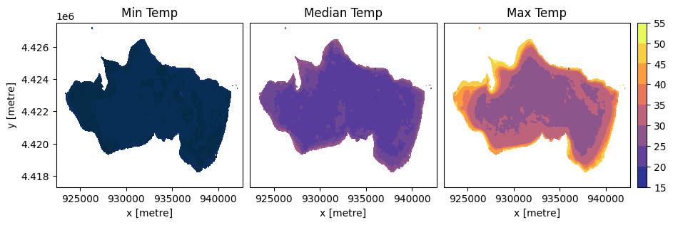
Water Temperature#
The surface water temperature, derived from the Thermal Infrared Sensor (TIRS) onboard Landsat-8 and Landsat-9, is a key variable influencing biological activity, stratification, and ecosystem dynamics. For each pixel, the 10th, 50th, and 90th percentiles of surface temperature measured in a year are recorded as the minimum, median, and maximum values. Below, we plot the surface temperature measurements for 2024.
[20]:
# Temperature variables to plot
temp_vars = ["tirs_st_ann_min", "tirs_st_ann_med", "tirs_st_ann_max"]
titles = ["Min Temp", "Median Temp", "Max Temp"]

# Shared min and max for colourbar
vmin = min(ds[v].sel(time="2024").min().item() for v in temp_vars)
vmax = max(ds[v].sel(time="2024").max().item() for v in temp_vars)

# Calculate figure size based on previous plot to preserve proportions
figsize_facetgrid = im.fig.get_size_inches()
panel_width = figsize_facetgrid[0] / len(im.axs.flat)
panel_height = figsize_facetgrid[1]

# Account for three plots and a colourbar
plot_ratios = [1, 1, 1]
colorbar_ratio = 0.05
total_ratio = sum(plot_ratios) + colorbar_ratio

figsize = (
    panel_width * total_ratio,
    panel_height
)

fig = plt.figure(figsize=figsize)

gs = GridSpec(
    1, 4,
    width_ratios=[1, 1, 1, 0.05],
    wspace=0.05
)

axs = [fig.add_subplot(gs[i]) for i in range(3)]
cax = fig.add_subplot(gs[3])

for ax, var, title in zip(axs, temp_vars, titles):
    im_temp = ds[var].sel(time="2024").squeeze().plot.contourf(
        ax=ax,
        cmap="cmo.thermal",
        vmin=vmin,
        vmax=vmax,
        add_colorbar=False
    )
    ax.set_title(title)

# Remove ylabel and yticks for 2nd and 3rd plot
for i, ax in enumerate(axs):
    if i > 0:
        ax.set_ylabel("")
        ax.set_yticks([])

# Shared colorbar
fig.colorbar(im_temp, cax=cax)

plt.show()
Yearly change monitoring#
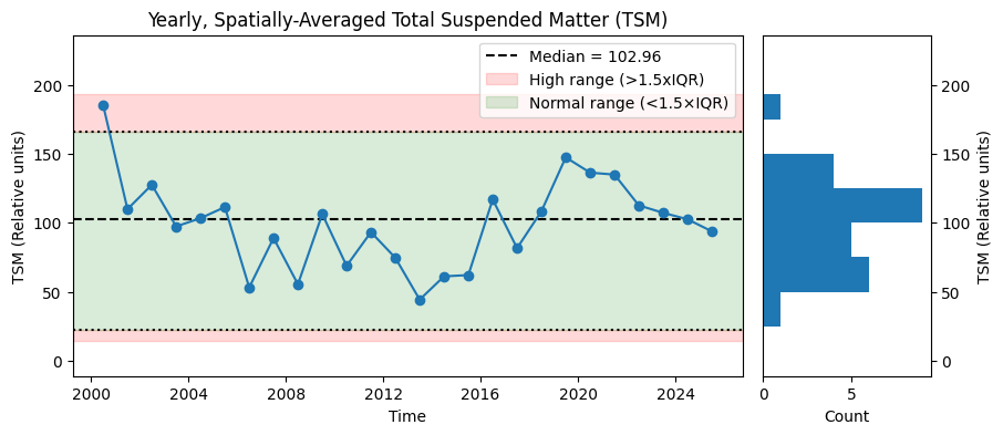
The annual water quality maps can be used to track year-to-year trends in water quality. We plot the spatial median of each yearly timestep as a time series. We also plot the interquartile ranges, demonstrating a simple method for anomaly detection.
[21]:
# Spatially-averaged time series
ts = ds.median(dim=["x", "y"])
vals = ts["tsm"].values

# Median
median_value = np.nanmedian(vals)

# IQR anomaly thresholds
q1 = np.nanpercentile(vals, 25)
q3 = np.nanpercentile(vals, 75)
iqr = q3 - q1

lower_bound = q1 - 1.5 * iqr
upper_bound = q3 + 1.5 * iqr

# Figure layout
fig = plt.figure(figsize=(10, 4))
gs = GridSpec(1, 2, width_ratios=[4, 1], wspace=0.05)

ax = fig.add_subplot(gs[0])
ax_hist = fig.add_subplot(gs[1], sharey=ax)

# Plot median of medians
ax.axhline(
    median_value, color="black", linestyle="--", label=f"Median = {median_value:.2f}"
)

# Plot time series
ts["tsm"].plot.line(ax=ax, marker="o")

# Plot IQR bounds
ax.axhline(lower_bound, color="black", linestyle=":")
ax.axhline(upper_bound, color="black", linestyle=":")

# Shade anomaly regions
ymin, ymax = ax.get_ylim()
ax.axhspan(ymin, lower_bound, color="red", alpha=0.15, label = "High range (>1.5xIQR)")
ax.axhspan(upper_bound, ymax, color="red", alpha=0.15)

# Shade normal region
ax.axhspan(
    lower_bound, upper_bound, color="green", alpha=0.15, label="Normal range (<1.5×IQR)"
)

# Labels
ax.set_title("Yearly, Spatially-Averaged Total Suspended Matter (TSM)")
ax.set_xlabel("Time")
ax.set_ylabel("TSM (Relative units)")
ax.legend()

# Align histogram bins to yticks
yticks = np.unique(ax.get_yticks())  # Remove duplicates
bins = np.sort(np.concatenate(([ymin], yticks, [ymax])))  # Ensure monotonic

ax_hist.hist(vals, bins=bins, orientation="horizontal")

# Histogram labels
ax_hist.set_xlabel("Count")
ax_hist.set_ylabel("TSM (Relative units)")
ax_hist.yaxis.set_label_position("right")
ax_hist.yaxis.tick_right()

plt.show()
Animation over time#
The annual maps can be visualised in an animation as demonstrated below using the xr_animation function. The interval parameter specifies the time in milliseconds between each image in the animation.
[22]:
# Calculate inverse scaling of data shape to remove spatial distortion
ny, nx = ds.tsm.isel(time=0).shape
inverse_data_aspect = nx / ny

xr_animation(
    ds,
    bands="tsm",
    output_path="water_quality.mp4",
    interval=500,
    show_date="%Y",
    annotation_kwargs={"fontsize": 28},
    imshow_kwargs={"cmap": "cmo.turbid", "aspect": inverse_data_aspect},
    colorbar_kwargs={"labelcolor": "black"}
)

plt.close()
Video(f"water_quality.mp4", embed=True)
Exporting animation to water_quality.mp4
[22]:
Water Quality Summaries#
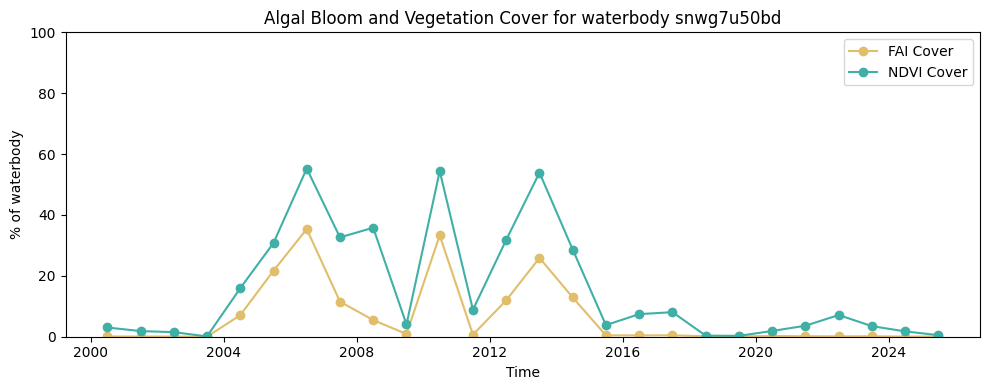
Together with the annual variables, the Water Quality Monitoring Service also provides per waterbody annual variable summaries for the over 700,000 waterbodies across the continent identified in the Waterbodies Service. The cell below demonstrates how to load the water quality summary for a waterbody.
For the NDVI and FAI variables, the summaries provided are ndvi_cover and fai_cover respectively. The ndvi_cover indicates the percentage of the waterbody that showed persistent vegetation cover throughout the year. The fai_cover indicates the percentage of the waterbody that showed persistent algal bloom cover throughout the year.
For the remaining variables i.e. hue (hue), optical water type (owt), median temperature (st_median), maximum temperature (st_max), minimum temperature (st_min), chlorophyll-a (chla), turbidity (tsm) and trophic state (ts), the value for each 10th percentile increment of a variable for a waterbody is provided.
The identifier for the waterbody can be found by loading the Waterbodies product in DE Africa Maps and clicking on the waterbody. Here is an example for Lake Ichkeul: https://maps.digitalearth.africa/#share=s-gVaEjpEAOcjPcUjX7N3oOxVBXnx
[23]:
# Waterbody uid for Lake Ichkeul
waterbody_uid = "snwg7u50bd"
waterbody = get_waterbody(waterbody_uid)
waterbody.explore()
[23]:
[24]:
wq_summary = get_water_quality_summary(waterbody_uid, start_date="2000-01-01", end_date="2025-12-31")
wq_summary.head()
[24]:
| hue_q0_1 | hue_q0_2 | hue_q0_3 | hue_q0_4 | hue_q0_5 | hue_q0_6 | hue_q0_7 | hue_q0_8 | hue_q0_9 | owt_q0_1 | ... | st_min_q0_2 | st_min_q0_3 | st_min_q0_4 | st_min_q0_5 | st_min_q0_6 | st_min_q0_7 | st_min_q0_8 | st_min_q0_9 | fai_cover | ndvi_cover | |
|---|---|---|---|---|---|---|---|---|---|---|---|---|---|---|---|---|---|---|---|---|---|
| date | |||||||||||||||||||||
| 2000-07-01 | 40.755914 | 42.516296 | 43.284092 | 43.759880 | 44.137211 | 44.484035 | 44.863377 | 45.323807 | 45.998134 | 1.0 | ... | 10.447911 | 11.090235 | 11.662890 | 12.091141 | 12.401832 | 12.697342 | 12.984018 | 13.412905 | 0.082582 | 3.034801 |
| 2001-07-02 | 43.807373 | 46.435708 | 47.598160 | 48.390659 | 49.231701 | 49.961061 | 50.539479 | 51.093925 | 51.751480 | 1.0 | ... | 11.765969 | 12.053548 | 12.345901 | 12.616390 | 12.846532 | 13.099591 | 13.426577 | 14.073029 | 0.066233 | 1.852661 |
| 2002-07-02 | 41.002720 | 43.746305 | 45.104209 | 46.083991 | 46.902491 | 47.673332 | 48.460795 | 49.372364 | 50.403860 | 1.0 | ... | 11.159149 | 11.305438 | 11.429169 | 11.546671 | 11.658873 | 11.790919 | 11.956471 | 12.315331 | 0.061111 | 1.502174 |
| 2003-07-02 | 48.976505 | 51.967916 | 53.384142 | 54.629906 | 55.841576 | 56.796713 | 57.683242 | 58.588321 | 59.644947 | 1.0 | ... | 11.747325 | 12.003418 | 12.260449 | 12.437958 | 12.604795 | 12.754241 | 12.938187 | 13.209305 | 0.004036 | 0.093451 |
| 2004-07-01 | 47.050282 | 48.767092 | 50.081455 | 51.027034 | 51.813360 | 52.556026 | 53.325633 | 54.222552 | 55.418394 | 1.0 | ... | 9.457001 | 9.807001 | 10.151760 | 10.605438 | 11.629942 | 12.435919 | 13.004912 | 13.464972 | 7.070729 | 15.904574 |
5 rows × 74 columns
[25]:
fig, ax = plt.subplots(figsize=(10, 4))
ax.plot(wq_summary.index, wq_summary["fai_cover"], color="#E1BE6A", linestyle="-", marker="o", label="FAI Cover")
ax.plot(wq_summary.index, wq_summary["ndvi_cover"], color="#40B0A6", linestyle="-", marker="o", label="NDVI Cover")
ax.set_xlabel("Time")
ax.set_ylim(0, 100)
ax.set_ylabel("% of waterbody")
ax.set_title(f"Algal Bloom and Vegetation Cover for waterbody {waterbody_uid}")
ax.legend()
plt.tight_layout()
plt.show()
The Water Quality Monitoring Service also provides a ranking for each waterbody compared to all other waterbodies in the Waterbodies Service. The service averages the water quality summary metrics: fai_cover, ndvi_cover, hue_q0_5, owt_q0_5, chla_q0_5, tsi_q0_5, tsm_q0_5, st_max_q0_5, st_median_q0_5 and st_min_q0_5 over the period 2020 – 2025 and provides a percentile ranking for each waterbody.
As can be seen below, Lake Ichkeul ranks highly for Total Suspended Matter (TSM) compared to other African waterbodies.
[26]:
wq_rank = get_water_quality_rankings(waterbody_uid)
wq_rank
[26]:
| fai_cover_percentile | ndvi_cover_percentile | hue_q0_5_percentile | owt_q0_5_percentile | chla_q0_5_percentile | tsi_q0_5_percentile | tsm_q0_5_percentile | st_max_q0_5_percentile | st_median_q0_5_percentile | st_min_q0_5_percentile | |
|---|---|---|---|---|---|---|---|---|---|---|
| 0 | 1.0 | 2.0 | 49.0 | 14.0 | 5.0 | 5.0 | 94.0 | 8.0 | 9.0 | 5.0 |
Informations Complémentaires#
Licence : Le code de ce carnet est sous licence Apache, version 2.0 <https://www.apache.org/licenses/LICENSE-2.0>. Les données de Digital Earth Africa sont sous licence Creative Commons par attribution 4.0 <https://creativecommons.org/licenses/by/4.0/>.
Contact : Si vous avez besoin d’aide, veuillez poster une question sur le canal Slack Open Data Cube <http://slack.opendatacube.org/>`__ ou sur le GIS Stack Exchange en utilisant la balise open-data-cube (vous pouvez consulter les questions posées précédemment ici). Si vous souhaitez signaler un problème avec ce bloc-notes, vous pouvez en déposer un sur Github.
Version de Datacube compatible :
[27]:
print(datacube.__version__)
1.9.13
Dernier test :
[28]:
from datetime import datetime

datetime.today().strftime("%Y-%m-%d")
[28]:
'2026-03-24'