Introduction to WaPOR and data loading

• Products used: WaPOR

Keywords data used; wapor data used; crop mask

Aperçu

The Water Productivity through Open access of Remotely sensed derived data (WaPOR) monitors and reports on agricultural water productivity through biophysical measures with a focus on Africa and the Near East. This information assists partner countries improve land and water productivity in both rainfed and irrigated agriculture (Peiser et al. 2017).

WaPOR provides numerous datasets related to vegetation productivity and water consumption, and associated meteorological and physical conditions such as soil moisture and precipitation. These datasets can be combined with Digital Earth Africa products, services, and workflows for numerous applications including:

• Suivi des conditions de sécheresse

• Suivi de l’efficacité de l’utilisation de l’eau par les cultures

• Cartographie des zones irriguées

• Estimation des besoins en eau des cultures

• Programmation et budgétisation de l’irrigation

Description

This notebook provides an introduction to WaPOR data and nomenclature, and demonstrates loading and plotting.

1. First, we explore the datasets available and how they are labelled.

2. Then, we download and plot annual evapotranspiration.

3. Finally, we download and plot dekadal (10 day temporal frequency) data.

---

Commencer

Pour exécuter cette analyse, exécutez toutes les cellules du bloc-notes, en commençant par la cellule « Charger les packages ».

Charger des paquets

Importez les packages Python utilisés pour l’analyse.

Use standard import commands; some are shown below. Begin with any iPython magic commands, followed by standard Python packages, then any additional functionality you need from the Tools package.

import datetime
import datacube
import geopandas as gpd

from deafrica_tools.load_wapor import get_all_WaPORv3_mapsets, get_WaPORv3_info, load_wapor_ds
from deafrica_tools.areaofinterest import define_area
from deafrica_tools.plotting import display_map
from wapordl import wapor_map
from odc.geo.geom import Geometry

INFO: WaPORDL (`1.0.2`)
WARNING: Latest version is '1.0.3'.
WARNING: Please update pywapor.

Se connecter au datacube

Connectez-vous au datacube pour que nous puissions accéder aux données de DE Africa. Le paramètre « app » est un nom unique pour l’analyse qui est basé sur le nom du fichier du notebook.

dc = datacube.Datacube(app="WaPOR")

WaPOR Data

Les données WaPOR comportent trois niveaux :

1. Résolution globale de 300 m

2. National 100m resolution

3. Résolution infranationale de 20 m

The table below covers L1 and L2 datasets. L3 datasets can be viewed in the WaPOR maps platform which is built with the same software as Digital Earth Africa Maps. L3 datasets cover several regions of interest in northern and eastern Africa. This notebook loads level 3 20m data for Egypt. It is recommended that the WaPOR maps platform is inspected to check the availability of level, variable, and temporal frequency combinations for your area of interest. The maps platform also shows map codes in the data description.

Mapset codes are structured as level-variable-temporal frequency as shown below. The temporal frequencies available are:

• A - annuel

• M - mensuel

• D - décadaire (10 jours)

So, for level 3 net primary productivity at dekadal intervals the code would be L3-NPP-D.

get_all_WaPORv3_mapsets()

	Mapset Code	Mapset Description
0	L1-AETI-A	Actual EvapoTranspiration and Interception (Gl...
1	L1-AETI-D	Actual EvapoTranspiration and Interception (Gl...
2	L1-AETI-M	Actual EvapoTranspiration and Interception (Gl...
3	L1-E-A	Evaporation (Global - Annual - 300m)
4	L1-E-D	Evaporation (Global - Dekadal - 300m)
5	L1-GBWP-A	Gross biomass water productivity (Annual - 300m)
6	L1-I-A	Interception (Global - Annual - 300m)
7	L1-I-D	Interception (Global - Dekadal - 300m)
8	L1-NBWP-A	Net biomass water productivity (Annual - 300m)
9	L1-NPP-D	Net Primary Production (Global - Dekadal - 300m)
10	L1-NPP-M	Net Primary Production (Global - Monthly - 300m)
11	L1-PCP-A	Precipitation (Global - Annual - Approximately...
12	L1-PCP-D	Precipitation (Global - Dekadal - Approximatel...
13	L1-PCP-E	Precipitation (Global - Daily - Approximately ...
14	L1-PCP-M	Precipitation (Global - Monthly - Approximatel...
15	L1-QUAL-LST-D	Quality land surface temperature (Global - Dek...
16	L1-QUAL-NDVI-D	Quality of Normalized Difference Vegetation In...
17	L1-RET-A	Reference Evapotranspiration (Global - Annual ...
18	L1-RET-D	Reference Evapotranspiration (Global - Dekadal...
19	L1-RET-E	Reference Evapotranspiration (Global - Daily -...
20	L1-RET-M	Reference Evapotranspiration (Global - Monthly...
21	L1-RSM-D	Relative Soil Moisture (Global - Dekadal - 300m)
22	L1-T-A	Transpiration (Global - Annual - 300m)
23	L1-T-D	Transpiration (Global - Dekadal - 300m)
24	L1-TBP-A	Total Biomass Production (Global - Annual - 300m)
25	L2-AETI-A	Actual EvapoTranspiration and Interception (Na...
26	L2-AETI-D	Actual EvapoTranspiration and Interception (Na...
27	L2-AETI-M	Actual EvapoTranspiration and Interception (Na...
28	L2-E-A	Evaporation (National - Annual - 100m)
29	L2-E-D	Evaporation (National - Dekadal - 100m)
30	L2-GBWP-A	Gross biomass water productivity (Annual - 100m)
31	L2-I-A	Interception (National - Annual - 100m)
32	L2-I-D	Interception (National - Dekadal - 100m)
33	L2-NBWP-A	Net biomass water productivity (Annual - 100m)
34	L2-NPP-D	Net Primary Production (National - Dekadal - 1...
35	L2-NPP-M	Net Primary Production (National - Monthly - 1...
36	L2-QUAL-NDVI-D	Quality of normalized difference vegetation in...
37	L2-RSM-D	Relative Soil Moisture (National - Dekadal - 1...
38	L2-T-A	Transpiration (National - Annual - 100m)
39	L2-T-D	Transpiration (National - Dekadal - 100m)
40	L2-TBP-A	Total Biomass Production (Global - Annual - 100m)

Paramètres d’analyse

The cell below specifies:

• The folder where the downloaded data will be stored. If you are using this script repeatedly, it is recommended you empty this folder from time to time to manage storage. It is advised that any data required for repeated or future analysis is stored outside the sandbox.

• The variable of interest in the form of a mapset code, explained above.

• The period of interest.

folder = "../Supplementary_data/WaPOR" # folder that the data will be sent to
variable = "L3-AETI-A" # level-variable-time, see table above
period = ["2018-01-01", "2024-02-01"] # period to load

Next, the area of interest is defined. This can also be a .geojson file which the loading function accepts. Otherwise, there are two methods available:

1. By specifying the latitude, longitude, and buffer. This method requires you to input the central latitude, central longitude, and the buffer value in square degrees around the center point you want to analyze. For example, lat = 30.75, lon = 31.35, and buffer = 0.1 will select an area with a radius of 0.1 square degrees around the point with coordinates (30.75, 31.35).

   Alternatively, you can provide separate buffer values for latitude and longitude for a rectangular area. For example, lat = 30.75, lon = 31.35, and lat_buffer = 0.1 andlon_buffer = 0.08 will select a rectangular area extending 0.1 degrees north and south, and 0.08 degrees east and west from the point (30.75, 31.35).

   Pour des temps de chargement raisonnables, définissez la mémoire tampon sur « 0,1 » ou moins.

2. By uploading a polygon as an Esri Shapefile. If you choose this option, you will need to upload the geojson or ESRI shapefile into the Sandbox using Upload Files button in the top left corner of the Jupyter Notebook interface. ESRI shapefiles must be uploaded with all the related files (.cpg, .dbf, .shp, .shx). Once uploaded, you can use the shapefile or geojson to define the area of interest. Remember to update the code to call the file you have uploaded.

Pour utiliser l’une de ces méthodes, vous pouvez décommenter la ligne de code concernée et commenter l’autre. Pour commenter une ligne, ajoutez le symbole "#" avant le code que vous souhaitez commenter. Par défaut, la première option qui définit l’emplacement à l’aide de la latitude, de la longitude et du tampon est utilisée.

Si vous exécutez le bloc-notes pour la première fois, conservez les paramètres par défaut ci-dessous. Cela permettra de démontrer le fonctionnement de l’analyse et de fournir des résultats significatifs.

# Method 1: Specify the latitude, longitude, and buffer
aoi = define_area(lat=30.75, lon=31.35, buffer=0.03)

# Method 2: Use a polygon as a GeoJSON or Esri Shapefile.
# aoi = define_area(vector_path='aoi.shp')

#Create a geopolygon and geodataframe of the area of interest
geopolygon = Geometry(aoi["features"][0]["geometry"], crs="epsg:4326")
geopolygon_gdf = gpd.GeoDataFrame(geometry=[geopolygon], crs=geopolygon.crs)

# Get the latitude and longitude range of the geopolygon
lat_range = (geopolygon_gdf.total_bounds[1], geopolygon_gdf.total_bounds[3])
lon_range = (geopolygon_gdf.total_bounds[0], geopolygon_gdf.total_bounds[2])

region = [geopolygon_gdf.total_bounds[0], geopolygon_gdf.total_bounds[1], geopolygon_gdf.total_bounds[2], geopolygon_gdf.total_bounds[3]]

This demonstration notebook loads an area of cropland in the Nile Delta, Egypt.

display_map(x=lon_range, y=lat_range)

Make this Notebook Trusted to load map: File -> Trust Notebook

Download netCDF files

This cell downloads the data specified. The aeti object is the file path to the stored netCDF. Once this cell is run, netCDF files will be stored in the directory specified above.

aeti = wapor_map(region, variable, period, folder, extension = '.nc')

WARNING: `region` intersects with multiple L3 regions (['ENO', 'ZAN']), continuing with ENO only.
INFO: Found 7 files for L3-AETI-A.
INFO: Converting from `.tif` to `.nc`.

Convert data to xarray

Below, the netCDFs are brought into the analysis environment as xarray datasets and coordinate labels and attributes are assigned. This means the data is in a common format with other Digital Earth Africa products and services, and makes the data easy to interact with. The load_wapor_ds() function brings in the data as xarray.

aeti_xr = load_wapor_ds(filename=aeti, variable=variable)

Inspect the xarray dataset

Now we have x, y, and time as dimensions and our variable (in this case, actual evapotranspiration and interception) as an xarray dataset. This enables us to easily deal with time and space for analysis.

aeti_xr

<xarray.Dataset> Size: 5MB
Dimensions:      (x: 294, y: 330, time: 7)
Coordinates:
  * x            (x) float64 2kB 3.391e+05 3.392e+05 ... 3.45e+05 3.45e+05
  * y            (y) float64 3kB 3.406e+06 3.406e+06 ... 3.4e+06 3.4e+06
    spatial_ref  int32 4B 32636
  * time         (time) datetime64[ns] 56B 2018-01-01 2019-01-01 ... 2024-01-01
Data variables:
    L3-AETI-A    (time, y, x) float64 5MB 1.234e+03 1.209e+03 ... 1.224e+03
Attributes:
    long_name:            Actual EvapoTranspiration and Interception
    overview:             NONE
    temporal_resolution:  Year
    units:                mm/year
    scale_factor:         0.1
    _FillValue:           -9999
    add_offset:           0.0

xarray.Dataset

• Dimensions:
  • x: 294
  • y: 330
  • time: 7
• Coordinates: (4)
  • x
    (x)
    float64
    3.391e+05 3.392e+05 ... 3.45e+05

    long_name :

    x coordinate of projection

    standard_name :

    projection_x_coordinate

    units :

    m

    array([339130., 339150., 339170., ..., 344950., 344970., 344990.])

  • y
    (y)
    float64
    3.406e+06 3.406e+06 ... 3.4e+06

    long_name :

    y coordinate of projection

    standard_name :

    projection_y_coordinate

    units :

    m

    array([3406350., 3406330., 3406310., ..., 3399810., 3399790., 3399770.])

  • spatial_ref
    ()
    int32
    32636

    spatial_ref :

    PROJCS["WGS 84 / UTM zone 36N",GEOGCS["WGS 84",DATUM["WGS_1984",SPHEROID["WGS 84",6378137,298.257223563,AUTHORITY["EPSG","7030"]],AUTHORITY["EPSG","6326"]],PRIMEM["Greenwich",0,AUTHORITY["EPSG","8901"]],UNIT["degree",0.0174532925199433,AUTHORITY["EPSG","9122"]],AUTHORITY["EPSG","4326"]],PROJECTION["Transverse_Mercator"],PARAMETER["latitude_of_origin",0],PARAMETER["central_meridian",33],PARAMETER["scale_factor",0.9996],PARAMETER["false_easting",500000],PARAMETER["false_northing",0],UNIT["metre",1,AUTHORITY["EPSG","9001"]],AXIS["Easting",EAST],AXIS["Northing",NORTH],AUTHORITY["EPSG","32636"]]

    crs_wkt :

    PROJCS["WGS 84 / UTM zone 36N",GEOGCS["WGS 84",DATUM["WGS_1984",SPHEROID["WGS 84",6378137,298.257223563,AUTHORITY["EPSG","7030"]],AUTHORITY["EPSG","6326"]],PRIMEM["Greenwich",0,AUTHORITY["EPSG","8901"]],UNIT["degree",0.0174532925199433,AUTHORITY["EPSG","9122"]],AUTHORITY["EPSG","4326"]],PROJECTION["Transverse_Mercator"],PARAMETER["latitude_of_origin",0],PARAMETER["central_meridian",33],PARAMETER["scale_factor",0.9996],PARAMETER["false_easting",500000],PARAMETER["false_northing",0],UNIT["metre",1,AUTHORITY["EPSG","9001"]],AXIS["Easting",EAST],AXIS["Northing",NORTH],AUTHORITY["EPSG","32636"]]

    semi_major_axis :

    6378137.0

    semi_minor_axis :

    6356752.314245179

    inverse_flattening :

    298.257223563

    reference_ellipsoid_name :

    WGS 84

    longitude_of_prime_meridian :

    0.0

    prime_meridian_name :

    Greenwich

    geographic_crs_name :

    WGS 84

    horizontal_datum_name :

    World Geodetic System 1984

    projected_crs_name :

    WGS 84 / UTM zone 36N

    grid_mapping_name :

    transverse_mercator

    latitude_of_projection_origin :

    0.0

    longitude_of_central_meridian :

    33.0

    false_easting :

    500000.0

    false_northing :

    0.0

    scale_factor_at_central_meridian :

    0.9996

    GeoTransform :

    339120.0 20.0 0.0 3406360.0 0.0 -20.0

    array(32636, dtype=int32)

  • time
    (time)
    datetime64[ns]
    2018-01-01 ... 2024-01-01

    array(['2018-01-01T00:00:00.000000000', '2019-01-01T00:00:00.000000000',
           '2020-01-01T00:00:00.000000000', '2021-01-01T00:00:00.000000000',
           '2022-01-01T00:00:00.000000000', '2023-01-01T00:00:00.000000000',
           '2024-01-01T00:00:00.000000000'], dtype='datetime64[ns]')

• Data variables: (1)
  • L3-AETI-A
    (time, y, x)
    float64
    1.234e+03 1.209e+03 ... 1.224e+03

    long_name :

    Actual EvapoTranspiration and Interception

    overview :

    NONE

    temporal_resolution :

    Year

    units :

    mm/year

    scale_factor :

    0.1

    _FillValue :

    -9999

    add_offset :

    0.0

    array([[[1234. , 1209. , 1182.8, ..., 1230.6, 1246.6, 1275.9],
            [1268.4, 1269.3, 1223.5, ..., 1370. , 1338.9, 1298.7],
            [1212.7, 1245.2, 1263.6, ..., 1330.4, 1330.9, 1302.9],
            ...,
            [1195.1,  952.1,  935.3, ...,  948.5,  921.7, 1061. ],
            [1211.8, 1133.7, 1014.9, ...,  899.7,  930.1, 1091.7],
            [1278.6, 1072.2,  853.1, ...,  865. ,  935. , 1132.2]],
    
           [[1340.2, 1310.6, 1315.5, ..., 1406.6, 1401.4, 1384. ],
            [1439.1, 1399.6, 1368.6, ..., 1391.2, 1407.4, 1415.7],
            [1348.4, 1403.9, 1373.9, ..., 1468.8, 1460.7, 1427.3],
            ...,
            [1128.1,  916.5,  994.7, ..., 1352.9, 1319.2, 1250.3],
            [1147.4, 1133.6, 1094.9, ..., 1336.4, 1297.8, 1261.3],
            [1281.9, 1078.9,  876. , ..., 1295.4, 1266.4, 1271.3]],
    
           [[1364.5, 1376.7, 1404.6, ..., 1423.8, 1433.8, 1447.6],
            [1222.5, 1289.2, 1334.2, ..., 1423.2, 1404.8, 1392.4],
            [1154.3, 1149.8, 1319.9, ..., 1275.1, 1248.5, 1231.2],
            ...,
    ...
            ...,
            [1071.1,  879.2, 1062.1, ..., 1302.6, 1285.4, 1361.4],
            [1123.3, 1186.3, 1106.9, ..., 1224.6, 1239.5, 1371.5],
            [1396.7, 1101.7,  855.4, ..., 1076.4, 1195.2, 1279.6]],
    
           [[1240.4, 1256.5, 1272.7, ..., 1316.8, 1308.4, 1310.7],
            [1200.9, 1229.1, 1305. , ..., 1318.8, 1356.5, 1391.8],
            [1200. , 1231. , 1372.3, ..., 1483.2, 1478.8, 1465.3],
            ...,
            [1236.7,  969.2, 1116.8, ..., 1308. , 1491.5, 1571.6],
            [1245.6, 1208.8, 1260.1, ..., 1271.9, 1524. , 1551.4],
            [1315. , 1113. ,  898. , ..., 1145.4, 1519.9, 1490.4]],
    
           [[1404.9, 1440.7, 1459.4, ..., 1338.7, 1353.9, 1357.8],
            [1237. , 1307.5, 1392.3, ..., 1362.4, 1373.8, 1406.3],
            [1232. , 1251.1, 1292.4, ..., 1416.7, 1403.3, 1413.8],
            ...,
            [1142.8,  910. , 1112.2, ..., 1374.1, 1488.1, 1373.5],
            [1174.2, 1204.9, 1201.4, ..., 1346.6, 1499.3, 1319.6],
            [1436.1, 1232.6,  871.3, ..., 1171.4, 1492. , 1224.5]]])

• Indexes: (3)
  • x
    PandasIndex

    PandasIndex(Index([339130.0, 339150.0, 339170.0, 339190.0, 339210.0, 339230.0, 339250.0,
           339270.0, 339290.0, 339310.0,
           ...
           344810.0, 344830.0, 344850.0, 344870.0, 344890.0, 344910.0, 344930.0,
           344950.0, 344970.0, 344990.0],
          dtype='float64', name='x', length=294))

  • y
    PandasIndex

    PandasIndex(Index([3406350.0, 3406330.0, 3406310.0, 3406290.0, 3406270.0, 3406250.0,
           3406230.0, 3406210.0, 3406190.0, 3406170.0,
           ...
           3399950.0, 3399930.0, 3399910.0, 3399890.0, 3399870.0, 3399850.0,
           3399830.0, 3399810.0, 3399790.0, 3399770.0],
          dtype='float64', name='y', length=330))

  • time
    PandasIndex

    PandasIndex(DatetimeIndex(['2018-01-01', '2019-01-01', '2020-01-01', '2021-01-01',
                   '2022-01-01', '2023-01-01', '2024-01-01'],
                  dtype='datetime64[ns]', name='time', freq=None))

• Attributes: (7)

  long_name :

  Actual EvapoTranspiration and Interception

  overview :

  NONE

  temporal_resolution :

  Year

  units :

  mm/year

  scale_factor :

  0.1

  _FillValue :

  -9999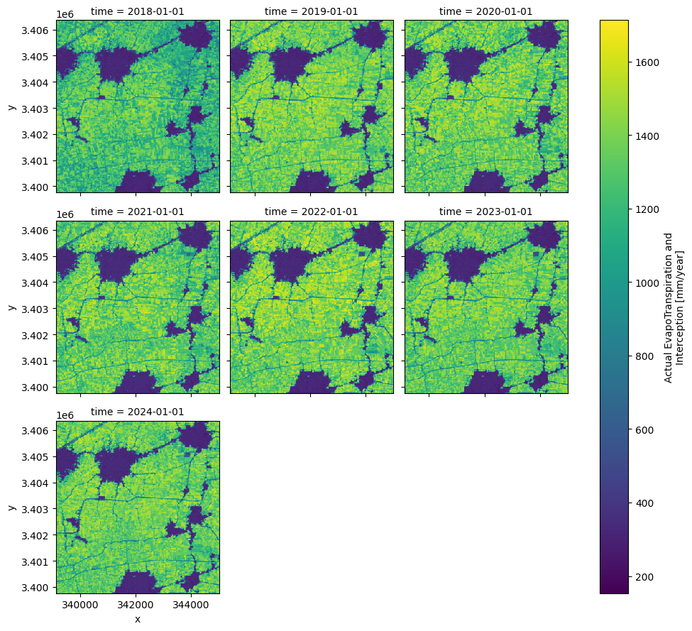

  add_offset :

  0.0

Plot annual ET

The plots show how AETI varies in space and between years. In the Egypt example, the cropland areas are easily visible as areas with higher AETI.

Note that the scalebar is labelled with information from the WaPOR metadata. This can be accessed by calling aeti_xr[variable].attrs, as below, which can be especially useful when checking units for calculation. The load_wapor_ds() function takes care of re-scaling when the data is loaded, but it is sensible to check the values are reasonable.

We can also see that the attributes include scale and offset values. These have been incorporated into the load_wapor_ds() function so the values returned are in the units shown below, in this case mm/year.

aeti_xr[variable].attrs

{'long_name': 'Actual EvapoTranspiration and Interception',
 'overview': 'NONE',
 'temporal_resolution': 'Year',
 'units': 'mm/year',
 'scale_factor': 0.1,
 '_FillValue': -9999,
 'add_offset': 0.0}

aeti_xr[variable].plot(col='time', col_wrap=3)

<xarray.plot.facetgrid.FacetGrid at 0x7f059bf1a8a0>

Load dekadal biomass

The cell below loads dekadal actual evapotranspiration using the same procedure as for annual. The only parameter changed is variable.

variable = 'L3-NPP-D'
period = ["2024-01-01", "2024-03-01"]

npp_d = wapor_map(region, variable, period, folder, extension = '.nc')

npp_d_xr = load_wapor_ds(filename=npp_d, variable=variable)

npp_d_xr

WARNING: `region` intersects with multiple L3 regions (['ENO', 'ZAN']), continuing with ENO only.
INFO: Found 7 files for L3-NPP-D.
INFO: Converting from `.tif` to `.nc`.

<xarray.Dataset> Size: 5MB
Dimensions:      (x: 294, y: 330, time: 7)
Coordinates:
  * x            (x) float64 2kB 3.391e+05 3.392e+05 ... 3.45e+05 3.45e+05
  * y            (y) float64 3kB 3.406e+06 3.406e+06 ... 3.4e+06 3.4e+06
    spatial_ref  int32 4B 32636
  * time         (time) datetime64[ns] 56B 2024-01-01 2024-01-11 ... 2024-03-01
Data variables:
    L3-NPP-D     (time, y, x) float64 5MB 5.136 5.059 4.966 ... 7.505 7.186
Attributes:
    long_name:            Net Primary Production
    overview:             NONE
    temporal_resolution:  Dekad
    units:                gC/m²/day
    scale_factor:         0.001
    _FillValue:           -9999
    add_offset:           0.0

xarray.Dataset

• Dimensions:
  • x: 294
  • y: 330
  • time: 7
• Coordinates: (4)
  • x
    (x)
    float64
    3.391e+05 3.392e+05 ... 3.45e+05

    long_name :

    x coordinate of projection

    standard_name :

    projection_x_coordinate

    units :

    m

    array([339130., 339150., 339170., ..., 344950., 344970., 344990.])

  • y
    (y)
    float64
    3.406e+06 3.406e+06 ... 3.4e+06

    long_name :

    y coordinate of projection

    standard_name :

    projection_y_coordinate

    units :

    m

    array([3406350., 3406330., 3406310., ..., 3399810., 3399790., 3399770.])

  • spatial_ref
    ()
    int32
    32636

    spatial_ref :

    PROJCS["WGS 84 / UTM zone 36N",GEOGCS["WGS 84",DATUM["WGS_1984",SPHEROID["WGS 84",6378137,298.257223563,AUTHORITY["EPSG","7030"]],AUTHORITY["EPSG","6326"]],PRIMEM["Greenwich",0,AUTHORITY["EPSG","8901"]],UNIT["degree",0.0174532925199433,AUTHORITY["EPSG","9122"]],AUTHORITY["EPSG","4326"]],PROJECTION["Transverse_Mercator"],PARAMETER["latitude_of_origin",0],PARAMETER["central_meridian",33],PARAMETER["scale_factor",0.9996],PARAMETER["false_easting",500000],PARAMETER["false_northing",0],UNIT["metre",1,AUTHORITY["EPSG","9001"]],AXIS["Easting",EAST],AXIS["Northing",NORTH],AUTHORITY["EPSG","32636"]]

    crs_wkt :

    PROJCS["WGS 84 / UTM zone 36N",GEOGCS["WGS 84",DATUM["WGS_1984",SPHEROID["WGS 84",6378137,298.257223563,AUTHORITY["EPSG","7030"]],AUTHORITY["EPSG","6326"]],PRIMEM["Greenwich",0,AUTHORITY["EPSG","8901"]],UNIT["degree",0.0174532925199433,AUTHORITY["EPSG","9122"]],AUTHORITY["EPSG","4326"]],PROJECTION["Transverse_Mercator"],PARAMETER["latitude_of_origin",0],PARAMETER["central_meridian",33],PARAMETER["scale_factor",0.9996],PARAMETER["false_easting",500000],PARAMETER["false_northing",0],UNIT["metre",1,AUTHORITY["EPSG","9001"]],AXIS["Easting",EAST],AXIS["Northing",NORTH],AUTHORITY["EPSG","32636"]]

    semi_major_axis :

    6378137.0

    semi_minor_axis :

    6356752.314245179

    inverse_flattening :

    298.257223563

    reference_ellipsoid_name :

    WGS 84

    longitude_of_prime_meridian :

    0.0

    prime_meridian_name :

    Greenwich

    geographic_crs_name :

    WGS 84

    horizontal_datum_name :

    World Geodetic System 1984

    projected_crs_name :

    WGS 84 / UTM zone 36N

    grid_mapping_name :

    transverse_mercator

    latitude_of_projection_origin :

    0.0

    longitude_of_central_meridian :

    33.0

    false_easting :

    500000.0

    false_northing :

    0.0

    scale_factor_at_central_meridian :

    0.9996

    GeoTransform :

    339120.0 20.0 0.0 3406360.0 0.0 -20.0

    array(32636, dtype=int32)

  • time
    (time)
    datetime64[ns]
    2024-01-01 ... 2024-03-01

    array(['2024-01-01T00:00:00.000000000', '2024-01-11T00:00:00.000000000',
           '2024-01-21T00:00:00.000000000', '2024-02-01T00:00:00.000000000',
           '2024-02-11T00:00:00.000000000', '2024-02-21T00:00:00.000000000',
           '2024-03-01T00:00:00.000000000'], dtype='datetime64[ns]')

• Data variables: (1)
  • L3-NPP-D
    (time, y, x)
    float64
    5.136 5.059 4.966 ... 7.505 7.186

    long_name :

    Net Primary Production

    overview :

    NONE

    temporal_resolution :

    Dekad

    units :

    gC/m²/day

    scale_factor :

    0.001

    _FillValue :

    -9999

    add_offset :

    0.0

    array([[[5.136, 5.059, 4.966, ..., 4.908, 4.962, 5.09 ],
            [5.135, 5.085, 4.093, ..., 5.061, 4.928, 4.791],
            [5.166, 4.824, 4.362, ..., 3.423, 3.154, 2.946],
            ...,
            [1.416, 1.84 , 2.875, ..., 5.131, 5.189, 4.782],
            [1.899, 2.69 , 3.183, ..., 5.151, 5.105, 4.897],
            [4.144, 2.989, 2.494, ..., 4.033, 4.918, 4.669]],
    
           [[4.789, 4.868, 4.795, ..., 4.642, 4.701, 4.829],
            [4.901, 4.903, 4.032, ..., 4.797, 4.705, 4.612],
            [4.888, 4.842, 4.389, ..., 3.51 , 3.236, 3.045],
            ...,
            [0.977, 1.554, 2.621, ..., 4.886, 4.901, 4.665],
            [1.506, 2.427, 2.898, ..., 4.855, 4.808, 4.76 ],
            [3.808, 2.713, 2.267, ..., 3.884, 4.642, 4.554]],
    
           [[3.824, 3.951, 3.887, ..., 3.697, 3.762, 3.851],
            [3.956, 3.957, 3.308, ..., 3.823, 3.77 , 3.674],
            [3.947, 3.943, 3.644, ..., 2.969, 2.74 , 2.579],
            ...,
    ...
            ...,
            [2.151, 1.951, 3.207, ..., 5.455, 5.466, 5.473],
            [2.605, 2.723, 3.611, ..., 5.467, 5.435, 5.46 ],
            [4.846, 2.769, 2.433, ..., 4.736, 5.114, 5.202]],
    
           [[6.868, 7.151, 7.123, ..., 6.538, 6.749, 6.972],
            [7.078, 7.097, 5.712, ..., 6.848, 6.801, 6.553],
            [6.949, 6.934, 6.479, ..., 5.955, 5.607, 5.297],
            ...,
            [3.595, 2.792, 4.125, ..., 7.131, 7.147, 7.104],
            [3.956, 3.614, 4.481, ..., 7.15 , 6.926, 6.934],
            [6.307, 3.565, 3.081, ..., 6.236, 6.583, 6.61 ]],
    
           [[8.164, 8.232, 8.227, ..., 7.096, 7.388, 7.714],
            [7.515, 7.798, 6.502, ..., 7.596, 7.534, 7.31 ],
            [7.092, 7.238, 6.692, ..., 6.84 , 6.504, 6.172],
            ...,
            [4.886, 3.476, 4.58 , ..., 8.032, 8.206, 7.671],
            [5.116, 4.26 , 4.875, ..., 8.227, 7.79 , 7.422],
            [7.189, 4.079, 3.394, ..., 7.012, 7.505, 7.186]]])

• Indexes: (3)
  • x
    PandasIndex

    PandasIndex(Index([339130.0, 339150.0, 339170.0, 339190.0, 339210.0, 339230.0, 339250.0,
           339270.0, 339290.0, 339310.0,
           ...
           344810.0, 344830.0, 344850.0, 344870.0, 344890.0, 344910.0, 344930.0,
           344950.0, 344970.0, 344990.0],
          dtype='float64', name='x', length=294))

  • y
    PandasIndex

    PandasIndex(Index([3406350.0, 3406330.0, 3406310.0, 3406290.0, 3406270.0, 3406250.0,
           3406230.0, 3406210.0, 3406190.0, 3406170.0,
           ...
           3399950.0, 3399930.0, 3399910.0, 3399890.0, 3399870.0, 3399850.0,
           3399830.0, 3399810.0, 3399790.0, 3399770.0],
          dtype='float64', name='y', length=330))

  • time
    PandasIndex

    PandasIndex(DatetimeIndex(['2024-01-01', '2024-01-11', '2024-01-21', '2024-02-01',
                   '2024-02-11', '2024-02-21', '2024-03-01'],
                  dtype='datetime64[ns]', name='time', freq=None))

• Attributes: (7)

  long_name :

  Net Primary Production

  overview :

  NONE

  temporal_resolution :

  Dekad

  units :

  gC/m²/day

  scale_factor :

  0.001

  _FillValue :

  -9999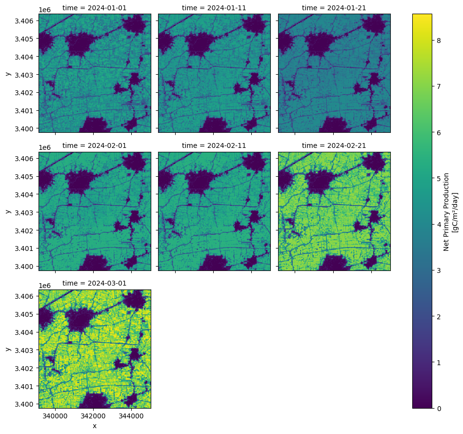

  add_offset :

  0.0

Plot dekadal net primary productivity

It’s interesting to note that in the Egypt example, some areas show very high biomass production > 30t/ha, especially in 2023. This must be considered in the context of several crop cycles occurring within a 12 month period.

npp_d_xr[variable].plot(col='time', col_wrap=3)

<xarray.plot.facetgrid.FacetGrid at 0x7f0599314c50>

Conclusion

This notebook demonstrated the range of WaPOR variables available and how to load them in the DE Africa Sandbox environment. Subsequent notebooks will dive deeper into analysing WaPOR data alongside DE Africa data.

---

Informations Complémentaires

Licence : Le code de ce carnet est sous licence Apache, version 2.0 <https://www.apache.org/licenses/LICENSE-2.0>. Les données de Digital Earth Africa sont sous licence Creative Commons par attribution 4.0 <https://creativecommons.org/licenses/by/4.0/>.

Contact : Si vous avez besoin d’aide, veuillez poster une question sur le canal Slack Open Data Cube <http://slack.opendatacube.org/>`__ ou sur le GIS Stack Exchange en utilisant la balise open-data-cube (vous pouvez consulter les questions posées précédemment ici). Si vous souhaitez signaler un problème avec ce bloc-notes, vous pouvez en déposer un sur Github.

Version de Datacube compatible :

print(datacube.__version__)

1.8.20

Dernier test :

from datetime import datetime
datetime.today().strftime('%Y-%m-%d')

'2025-02-17'