Sentinel-3 OLCI Land

Products used: s3_olci_l2_lfr

Keywords data used; sentinel-3,:index:datasets; sentinel-3

Aperçu

The Sentinel-3 OLCI Level-2 Land Full Resolution (OL_2_LFR) product provides atmospherically corrected observations and biophysical parameters derived from the Ocean and Land Colour Instrument (OLCI) onboard Sentinel-3A and 3B satellites. The product delivers consistent measurements of vegetation condition and atmospheric properties at 300-m resolution with an approximately daily revisit frequency with both satellites combined, making it valuable for a wide range of environmental and agricultural applications, including:

Vegetation health and stress monitoring
Drought early warning and food security assessments
Land surface process and ecosystem modelling
Crop condition analysis and agricultural productivity studies
Phenology and seasonal dynamics monitoring
Climate and atmospheric studies (via integrated water vapour)
Long-term land cover and change mapping

The algorithms and retrieval approaches have been developed by the European Space Agency (ESA) and partners, ensuring continuity with MERIS heritage and improved spectral and radiometric performance. Validation draws on ground-based measurements and inter-comparison with other satellite products. More information on the product can be found in the OLCI Land User Guide and Algorithm Theoretical Basis Documents (ATBDs). ***

Description

Ce cahier couvrira les sujets suivants :

Inspection des produits et des mesures disponibles dans le datacube
Loading Sentinel-3 OLCI Data.
Plotting the results

Commencer

Pour exécuter cette analyse, exécutez toutes les cellules du bloc-notes, en commençant par la cellule « Charger les packages ».

Charger des paquets

Importez les packages Python utilisés pour l’analyse.

[1]:

%matplotlib inline

import datacube
import geopandas as gpd
from odc.geo.geom import Geometry

from deafrica_tools.plotting import display_map
from deafrica_tools.areaofinterest import define_area

Se connecter au datacube

Connectez-vous au datacube pour que nous puissions accéder aux données de DE Africa.

[2]:

dc = datacube.Datacube(app="Sentinel_3")

Liste des produits

We can use datacube’s list_products functionality to inspect DE Africa’s products that are available in the datacube. The table below shows the product names that we will use to load the data, a brief description of the data, and the satellite instrument that acquired the data.

[3]:

dc.list_products().loc[dc.list_products()['description'].str.contains('Sentinel-3')]

[3]:

	name	description	license	default_crs	default_resolution
name
s3_ol_2_wfr_nrt	s3_ol_2_wfr_nrt	Sentinel-3 Level 2 Water Full Resolution (WFR)...	CC-BY-4.0	EPSG:4326	(-0.003, 0.003)
s3_olci_l2_lfr	s3_olci_l2_lfr	Sentinel-3 OLCI L2 LAND	CC-BY-4.0	EPSG:4326	(-0.003, 0.003)

Please choose the product by specifying its name, with the product s3_olci_l2_lfr

[4]:

product = "s3_olci_l2_lfr"

Liste des mesures

We can further inspect the data available for the Sentinel-3 Land s3_olci_l2_lfr product using datacube’s list_measurements functionality. The table below lists each of the measurements available in the data.

[5]:

measurements = dc.list_measurements()
measurements.loc[product]

[5]:

	name	dtype	units	nodata	aliases	flags_definition	add_offset	scale_factor
measurement
GIFAPAR	GIFAPAR	uint16	1	65535	[GI-FAPAR]	NaN	0.0	10000.0
IWV_L	IWV_L	uint8	kg/m²	255	[water_vapour]	NaN	0.0	1.0
OTCI	OTCI	uint16	1	65535	[chlorophyll]	NaN	0.0	10000.0
RC681	RC681	uint16	1	65535	NaN	NaN	0.0	10000.0
RC865	RC865	uint16	1	65535	NaN	NaN	0.0	10000.0
LQSF	LQSF	float32	1	-1	NaN	NaN	0.0	1.0
dataMask	dataMask	uint8	1	255	[mask]	NaN	0.0	1.0

The Sentinel-3 Land product has seven measurements:

Measurement	Description	Application
GIFAPAR (Green Instantaneous FAPAR)	Fraction of Absorbed Photosynthetically Active Radiation (green component) at observation time. Indicates photosynthetic energy uptake.	Vegetation productivity monitoring, drought early warning, crop and forest condition assessment.
IWV_L (Integrated Water Vapour – Land)	Column-integrated water vapour content above each pixel.	Climate modelling, evapotranspiration studies, vegetation stress analysis.
OTCI (OLCI Terrestrial Chlorophyll Index)	Index sensitive to canopy chlorophyll content derived from OLCI spectral bands.	Crop stress detection, canopy functioning studies, biomass dynamics monitoring.
RC681 (Rectified Reflectance 681 nm)	Atmospherically corrected surface reflectance in the red band (681 nm).	Input for vegetation indices and biophysical parameter retrievals.
RC865 (Rectified Reflectance 865 nm)	Atmospherically corrected surface reflectance in the NIR band (865 nm).	Used with RC681 for GIFAPAR; vegetation monitoring and photosynthetic activity modelling.
LQSF (Land Quality & Science Flags)	Per-pixel quality and classification information (land/water/cloud/snow).	Masking invalid pixels, cloud/snow filtering, ensuring robust time-series analysis.
dataMask	Binary mask indicating valid vs. invalid observations.	Excluding missing/invalid values, ensuring reliable data analysis.

Paramètres d’analyse

La cellule suivante définit les paramètres qui définissent la zone d’intérêt sur laquelle effectuer l’analyse. #### Sélectionner l’emplacement Pour définir la zone d’intérêt, deux méthodes sont disponibles :

En spécifiant la latitude, la longitude et la zone tampon, ou en séparant les zones tampons de latitude et de longitude, cette méthode vous permet de définir une zone d’intérêt autour d’un point central. Vous pouvez saisir la latitude centrale, la longitude centrale et une valeur de zone tampon en degrés pour créer une zone carrée autour du point central. Par exemple, « lat = 10.338 », « lon = -1.055 » et « buffer = 0.1 » sélectionneront une zone avec un rayon de 0,1 degré carré autour du point avec les coordonnées « (10.338, -1.055) ».

Vous pouvez également fournir des valeurs de tampon distinctes pour la latitude et la longitude d’une zone rectangulaire. Par exemple, « lat = 10.338 », « lon = -1.055 » et « lat_buffer = 0.1 » et « lon_buffer = 0.08 » sélectionneront une zone rectangulaire s’étendant sur 0,1 degré au nord et au sud et 0,08 degré à l’est et à l’ouest à partir du point « (10.338, -1.055) ».

Pour des temps de chargement raisonnables, définissez la mémoire tampon sur « 0,1 » ou moins.
By uploading a polygon as a GeoJSON or Esri Shapefile. If you choose this option, you will need to upload the geojson or ESRI shapefile into the Sandbox using Upload Files button in the top left corner of the Jupyter Notebook interface. ESRI shapefiles must be uploaded with all the related files (.cpg, .dbf, .shp, .shx). Once uploaded, you can use the shapefile or geojson to define the area of interest. Remember to update the code to call the file you have uploaded.

Pour utiliser l’une de ces méthodes, vous pouvez décommenter la ligne de code concernée et commenter l’autre. Pour commenter une ligne, ajoutez le symbole "#" avant le code que vous souhaitez commenter. Par défaut, la première option qui définit l’emplacement à l’aide de la latitude, de la longitude et du tampon est utilisée.

If running the notebook for the first time, keep the default settings below. This will demonstrate how the analysis works and provide meaningful results. The example covers a central Congo Basin belt (evergreen lowland rainforest) in Democratic Republic of the Congo (DRC), northeastern part of the country—within Tshopo Province. This region is characterised by frequent, heavy cloud cover so is often difficult to monitor effectively with optical missions that have lower revisit frequency, such as the Sentinel and Landsat missions.

To run the notebook for a different area, make sure Sentinel-3 OLCI Land data is available for the chosen area using the DEAfrica Explorer.

[6]:

# Method 1: Specify the latitude, longitude, and buffer)
aoi = define_area(lat=1.066, lon=26.455, buffer=0.9)

# Method 2: Use a polygon as a GeoJSON or Esri Shapefile.
# aoi = define_area(vector_path='aoi.shp')

#Create a geopolygon and geodataframe of the area of interest
geopolygon = Geometry(aoi["features"][0]["geometry"], crs="epsg:4326")
geopolygon_gdf = gpd.GeoDataFrame(geometry=[geopolygon], crs=geopolygon.crs)

# Get the latitude and longitude range of the geopolygon
lat_range = (geopolygon_gdf.total_bounds[1], geopolygon_gdf.total_bounds[3])
lon_range = (geopolygon_gdf.total_bounds[0], geopolygon_gdf.total_bounds[2])

[7]:

display_map(x=lon_range, y=lat_range)

[7]:

Make this Notebook Trusted to load map: File -> Trust Notebook

Masquage

Before visualisation, we use the dataMask band to mask values affected by cloud or other issues. The code below keeps data for pixels where the data mask value is 1.

[9]:

ds_S3 = ds_S3.where(ds_S3.dataMask == 1)

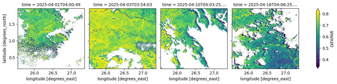
The cell below visualizes the Fraction of Absorbed Photosynthetically Active Radiation (green component) at the time of observation, which represents photosynthetic energy uptake. Values range from 0 to 1.

[10]:

(ds_S3['GIFAPAR'].isel(time=[0, 2, 9, 15])*0.0001).plot(robust=True, col="time", col_wrap=4);

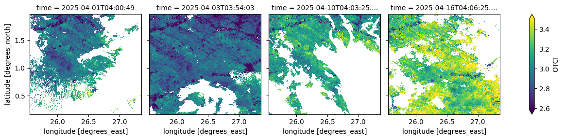
../../../_images/sandbox_notebooks_Datasets_Sentinel_3_Land_27_0.png

The cell below visualizes the OLCI Terrestrial Chlorophyll Index (OTCI), an index sensitive to canopy chlorophyll content derived from OLCI spectral bands. It provides information on vegetation health and photosynthetic activit

[11]:

(ds_S3.isel(time=[0, 2, 9, 15])['OTCI']*0.0001).plot(robust=True, col="time", col_wrap=4)

[11]:

<xarray.plot.facetgrid.FacetGrid at 0x7fa00b306d80>

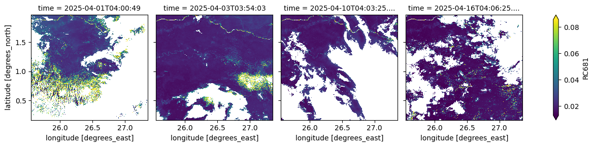
../../../_images/sandbox_notebooks_Datasets_Sentinel_3_Land_29_1.png

The cell below visualizes the atmospherically corrected surface reflectance in the red band (681 nm). This measurement is used in vegetation indices and biophysical parameter retrievals,

[12]:

(ds_S3.isel(time=[0, 2, 9, 15])['RC681']*0.0001).plot(robust=True, col="time", col_wrap=4)

[12]:

<xarray.plot.facetgrid.FacetGrid at 0x7fa0011924e0>

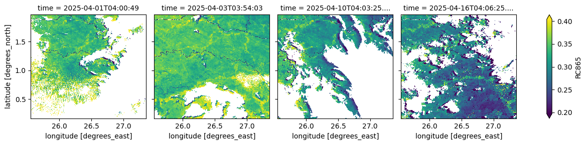
../../../_images/sandbox_notebooks_Datasets_Sentinel_3_Land_31_1.png

The cell below visualizes the atmospherically corrected surface reflectance in the near-infrared band (865 nm). This measurement, used alongside the red band (681 nm), supports vegetation monitoring and photosynthetic activity modelling,

[13]:

(ds_S3.isel(time=[0, 2, 9, 15])['RC865']*0.0001).plot(robust=True, col="time", col_wrap=4)

[13]:

<xarray.plot.facetgrid.FacetGrid at 0x7fa00b349f70>

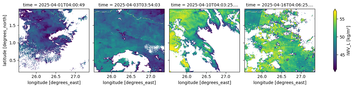
../../../_images/sandbox_notebooks_Datasets_Sentinel_3_Land_33_1.png

The cell below visualizes the column-integrated water vapour content above each pixel. This parameter represents the total amount of water vapour in the atmosphere, expressed in kg/m².

[14]:

(ds_S3.isel(time=[0, 2, 9, 15])['IWV_L']).plot(robust=True, col="time", col_wrap=4)

[14]:

<xarray.plot.facetgrid.FacetGrid at 0x7fa00b4be180>

../../../_images/sandbox_notebooks_Datasets_Sentinel_3_Land_35_1.png

Informations Complémentaires

Licence Le code de ce notebook est sous licence Apache, version 2.0 <https://www.apache.org/licenses/LICENSE-2.0>`__.

Les données de Digital Earth Africa sont sous licence Creative Commons Attribution 4.0 <https://creativecommons.org/licenses/by/4.0/>.

Contact Si vous avez besoin d’aide, veuillez poster une question sur le canal Slack DE Africa <https://digitalearthafrica.slack.com/> ou sur le GIS Stack Exchange <https://gis.stackexchange.com/questions/ask?tags=open-data-cube> en utilisant la balise open-data-cube (vous pouvez consulter les questions posées précédemment `ici <https://gis.stackexchange.com/questions/tagged/open-data-

Si vous souhaitez signaler un problème avec ce notebook, vous pouvez en déposer un sur Github.

Version de Datacube compatible

[15]:

print(datacube.__version__)

1.8.20

Dernier test :

[16]:

from datetime import datetime
datetime.today().strftime('%Y-%m-%d')

[16]:

'2025-09-16'