Mapping water extent and rainfall using Sentinel-1 and CHIRPS¶

Products used: s1_rtc, rainfall_chirps_monthly

**Keywords**: :index:`data used; sentinel-1`, :index:`data used; CHIRPS`, :index:`water; extent`, :index:`analysis; time series`

Contexte¶

The United Nations have prescribed 17 « Sustainable Development Goals » (SDGs). This notebook attempts to monitor SDG Indicator 6.6.1 - change in the extent of water-related ecosystems. Indicator 6.6.1 has 4 sub-indicators:

i. The spatial extent of water-related ecosystems
ii. The quantity of water contained within these ecosystems
iii. The quality of water within these ecosystems
iv. The health or state of these ecosystems

This notebook primarily focuses on the first sub-indicator - spatial extents.

Description¶

The notebook loads Sentinel-1 data, and using the sentinel-water-index, maps the spatial extent of water bodies. It also loads and plots monthly total rainfall from CHIRPS. The last section will compare the water extent between two periods to allow visulazing where change is occuring.

Load packages¶

Import Python packages that are used for the analysis.

[1]:

%matplotlib inline

import datacube
import xarray as xr
import numpy as np
import matplotlib.pyplot as plt

from deafrica_tools.datahandling import load_ard
from deafrica_tools.dask import create_local_dask_cluster
from deafrica_tools.datahandling import wofs_fuser

from long_term_water_extent import (
    load_vector_file,
    get_resampled_labels,
    resample_water_observations,
    resample_rainfall_observations,
    calculate_change_in_extent,
    compare_extent_and_rainfall,
)

Set up a Dask cluster¶

Dask can be used to better manage memory use and conduct the analysis in parallel.

[ ]:

create_local_dask_cluster()

Connect to Data Cube¶

[3]:

dc = datacube.Datacube(app="long_term_water_extent")

Analysis parameters¶

The following cell sets the parameters, which define the area of interest and the length of time to conduct the analysis over.

Upload a vector file for your water extent and your catchment to the data folder.
Set the time range you want to use.
Set the resampling strategy. Possible options include:
- "1Y" - Annual resampling, use this option for longer term monitoring
- "QS-DEC" - Quarterly resampling from December
- "3M" - Three-monthly resampling
- "1M" - Monthly resampling

For more details on resampling timeframes, see the xarray and pandas documentation.

[4]:

water_extent_vector_file = "data/lake_baringo_extent.geojson"

water_catchment_vector_file = "data/lake_baringo_catchment.geojson"

time_range = ("2018-07", "2021") #earliest date of S1 is July 1st 2018

resample_strategy = "Q-DEC"

dask_chunks = dict(x=1000, y=1000)

Get waterbody and catchment geometries¶

The next cell will extract the waterbody and catchment geometries from the supplied vector files, which will be used to load Water Observations from Space and the CHIRPS rainfall products.

[5]:

extent, extent_geometry = load_vector_file(water_extent_vector_file)
catchment, catchment_geometry = load_vector_file(water_catchment_vector_file)

Load Sentinel-1 for Waterbody¶

The first step is to load the Sentinel-1 data using the extent geometry.

[6]:

extent_query = {
    "time": time_range,
    "resolution": (-20, 20),
    "output_crs": "EPSG:6933",
    "geopolygon": extent_geometry,
    "group_by": "solar_day",
    "dask_chunks":dask_chunks
}

ds = load_ard(dc=dc, products=["s1_rtc"], measurements=["vv", "vh"], **extent_query)

Using pixel quality parameters for Sentinel 1
Finding datasets
    s1_rtc
Applying pixel quality/cloud mask
Returning 197 time steps as a dask array

Convert the Sentinel-1 digital numbers to dB¶

While Sentinel-1 backscatter is provided as linear intensiy, it is often useful to convert the backscatter to decible (dB) for analysis. Backscatter in dB unit has a more symmetric noise profile and less skewed value distribution for easier statistical evaluation.

The Sentinel-1 backscatter data is converted from digital number (DN) to backscatter in decibel unit (dB) using the function:

\begin{equation} 10 * \log_{10}(\text{DN}) \end{equation}

[7]:

# Convert DN to db values.
ds["vv_db"] = 10 * np.log10(ds.vv)
ds["vh_db"] = 10 * np.log10(ds.vh)

Calculate the SWI water index¶

The Sentinel-1A water index (SWI) is calculated as follows:

\begin{equation} \text{SWI} = 0.1747 * \beta _{vv} + 0.0082 * \beta _{vh} * \beta _{vv} + 0.0023 * \beta _{vv}^{2} - 0.0015 * \beta _{vh}^{2} + 0.1904 \end{equation}

where βvh and βvv represent the backscattering coefficient in VH polarization and VV polarization, respectively (Tian et al., 2017).

[8]:

# Calculate the Sentinel-1A Water Index (SWI).
ds['swi'] = (
    (0.1747 * ds.vv_db)
    + (0.0082 * ds.vh_db * ds.vv_db)
    + (0.0023 * ds.vv_db ** 2)
    - (0.0015 * ds.vh_db ** 2)
    + 0.1904
)

swi = ds[['swi']]
print(swi)

<xarray.Dataset>
Dimensions:      (time: 197, y: 1818, x: 852)
Coordinates:
  * time         (time) datetime64[ns] 2018-07-01T15:56:48.569171 ... 2021-12...
  * y            (y) float64 9.433e+04 9.431e+04 ... 5.801e+04 5.799e+04
  * x            (x) float64 3.473e+06 3.473e+06 3.473e+06 ... 3.49e+06 3.49e+06
    spatial_ref  int32 6933
Data variables:
    swi          (time, y, x) float32 dask.array<chunksize=(1, 1000, 852), meta=np.ndarray>
Attributes:
    crs:           EPSG:6933
    grid_mapping:  spatial_ref

Identify water in each resampling period¶

The second step is to resample the observations to get a consistent measure of the waterbody, and then calculate the classified as water for each period.

[9]:

resampled_water_ds, resampled_water_area_ds = resample_water_observations(
    swi, resample_strategy, radar=True
)

date_range_labels = get_resampled_labels(ds, resample_strategy)

/usr/local/lib/python3.10/dist-packages/dask/core.py:119: RuntimeWarning: divide by zero encountered in log10
  return func(*(_execute_task(a, cache) for a in args))
/usr/local/lib/python3.10/dist-packages/dask/core.py:119: RuntimeWarning: divide by zero encountered in log10
  return func(*(_execute_task(a, cache) for a in args))
/usr/local/lib/python3.10/dist-packages/dask/core.py:119: RuntimeWarning: invalid value encountered in add
  return func(*(_execute_task(a, cache) for a in args))
/usr/local/lib/python3.10/dist-packages/dask/core.py:119: RuntimeWarning: divide by zero encountered in log10
  return func(*(_execute_task(a, cache) for a in args))
/usr/local/lib/python3.10/dist-packages/dask/core.py:119: RuntimeWarning: invalid value encountered in subtract
  return func(*(_execute_task(a, cache) for a in args))
/usr/local/lib/python3.10/dist-packages/dask/core.py:119: RuntimeWarning: divide by zero encountered in log10
  return func(*(_execute_task(a, cache) for a in args))
/usr/local/lib/python3.10/dist-packages/dask/core.py:119: RuntimeWarning: invalid value encountered in add
  return func(*(_execute_task(a, cache) for a in args))
/usr/local/lib/python3.10/dist-packages/dask/core.py:119: RuntimeWarning: invalid value encountered in subtract
  return func(*(_execute_task(a, cache) for a in args))
/usr/local/lib/python3.10/dist-packages/dask/core.py:119: RuntimeWarning: divide by zero encountered in log10
  return func(*(_execute_task(a, cache) for a in args))
/usr/local/lib/python3.10/dist-packages/dask/core.py:119: RuntimeWarning: invalid value encountered in add
  return func(*(_execute_task(a, cache) for a in args))
/usr/local/lib/python3.10/dist-packages/dask/core.py:119: RuntimeWarning: invalid value encountered in subtract
  return func(*(_execute_task(a, cache) for a in args))
/usr/local/lib/python3.10/dist-packages/dask/core.py:119: RuntimeWarning: divide by zero encountered in log10
  return func(*(_execute_task(a, cache) for a in args))
/usr/local/lib/python3.10/dist-packages/dask/core.py:119: RuntimeWarning: invalid value encountered in subtract
  return func(*(_execute_task(a, cache) for a in args))
/usr/local/lib/python3.10/dist-packages/rasterio/warp.py:344: NotGeoreferencedWarning: Dataset has no geotransform, gcps, or rpcs. The identity matrix will be returned.
  _reproject(

Automatic SWI threshold: 0.59

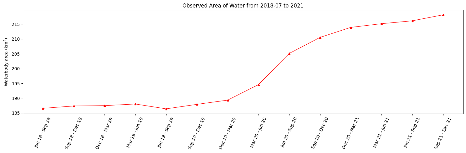
Plot the change in water area over time¶

[10]:

fig, ax = plt.subplots(figsize=(15, 5))

ax.plot(
    date_range_labels,
    resampled_water_area_ds.values,
    color="red",
    marker="^",
    markersize=4,
    linewidth=1,
)
plt.xticks(date_range_labels, rotation=65)
plt.title(f"Observed Area of Water from {time_range[0]} to {time_range[1]}")
plt.ylabel("Waterbody area (km$^2$)")
plt.tight_layout()

../../../../_images/sandbox_notebooks_Use_cases_Monitoring_water_extent_Monitoring_water_extent_radar_25_0.png

Load CHIRPS monthly rainfall¶

[11]:

catchment_query = {
    "time": time_range,
    "resolution": (-5000, 5000),
    "output_crs": "EPSG:6933",
    "geopolygon": catchment_geometry,
    "group_by": "solar_day",
    "dask_chunks":dask_chunks
}

rainfall_ds = dc.load(product="rainfall_chirps_monthly", **catchment_query)

Resample to estimate rainfall for each time period¶

This is done by taking calculating the average rainfall over the extent of the catchment, then summing these averages over the resampling period to estimate the total rainfall for the catchment.

[12]:

catchment_rainfall_resampled_ds = resample_rainfall_observations(
    rainfall_ds, resample_strategy, catchment
)

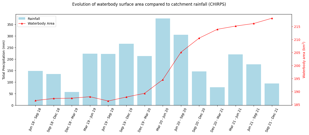
Compare waterbody area to catchment rainfall¶

This step plots the summed average rainfall for the catchment area over each period as a histogram, overlaid with the waterbody area calculated previously.

[13]:

figure = compare_extent_and_rainfall(
    resampled_water_area_ds, catchment_rainfall_resampled_ds, "mm", date_range_labels
)

../../../../_images/sandbox_notebooks_Use_cases_Monitoring_water_extent_Monitoring_water_extent_radar_31_0.png

Save the figure¶

[14]:

figure.savefig("waterarea_and_rainfall_radar.png", bbox_inches="tight")

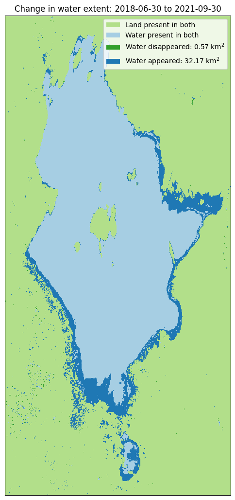
Compare water extent for two different periods¶

For the next step, enter a baseline date, and an analysis date to construct a plot showing where water appeared, as well as disappeared, by comparing the two dates.

[15]:

baseline_time = "2018-07-01"
analysis_time = "2021-10-01"

[16]:

figure = calculate_change_in_extent(baseline_time, analysis_time, resampled_water_ds, radar=True)

../../../../_images/sandbox_notebooks_Use_cases_Monitoring_water_extent_Monitoring_water_extent_radar_36_0.png

Save figure¶

[17]:

figure.savefig("waterarea_change_radar.png", bbox_inches="tight")

Additional information¶

License: The code in this notebook is licensed under the Apache License, Version 2.0. Digital Earth Africa data is licensed under the Creative Commons by Attribution 4.0 license.

Contact: If you need assistance, please post a question on the Open Data Cube Slack channel or on the GIS Stack Exchange using the open-data-cube tag (you can view previously asked questions here). If you would like to report an issue with this notebook, you can file one on Github.

Compatible datacube version:

[18]:

print(datacube.__version__)

1.8.15

Last Tested:

[19]:

from datetime import datetime
datetime.today().strftime('%Y-%m-%d')

[19]:

'2023-08-21'